
Train vs Plane vs Car: Emissions Methodology and Modal Comparison Approach

Every “the train is greener than flying” claim rests on a comparison that is, as usually presented, arithmetically invalid — a car factor quoted per vehicle-kilometre set against a rail factor quoted per passenger-kilometre, with radiative forcing silently included on one mode and excluded on another.
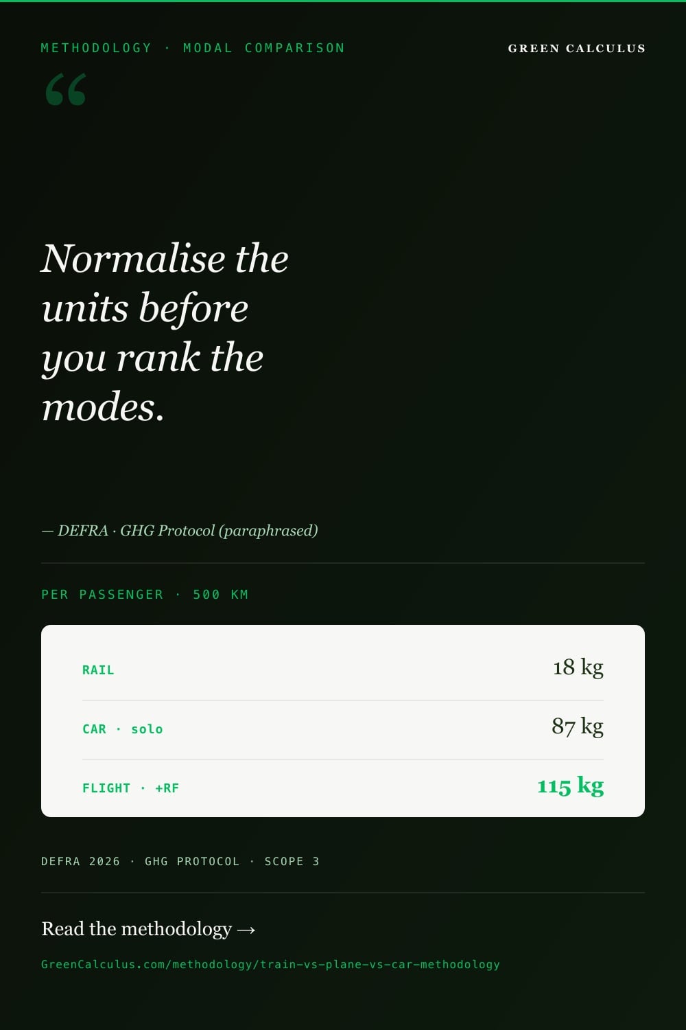
Normalise the units, fix the occupancy assumption, and decide the radiative-forcing question before you rank anything — the ordering is not stable until you do.
Per passenger-kilometre under DEFRA 2026 factors, national rail is the lowest-carbon mode, a domestic flight the highest, and car in between. Both of those rankings flip: the car on occupancy, the flight on whether radiative forcing is applied.
This page is the calculation reference for comparing passenger rail, air, and car on a like-for-like carbon basis. It sets out the emission-factor source for each mode, the four conventions that move the ranking, the normalisation chain that converts three incompatible unit bases into one comparable figure, and three hardcoded worked journeys that show the ranking changing under realistic inputs. It is written for the practitioner deciding which mode to book, which mode to report, and how to defend the number at reasonable-assurance review.
Provider directory
Now it has to hold up all year.
See who does this work. Every listing names the standards it works to, and paid placements are labelled. Including The Carbon Trust and Pangolin Associates.
Browse 6 carbon accounting & inventory providers →Do this work? A listing is US$390 a year. Get listed →
The Comparability Problem: Why Modal Factors Don’t Compare Directly
The three modes are published on three different denominators. A DEFRA car factor is expressed per vehicle-kilometre — it does not care how many people are in the car. A DEFRA rail or air factor is expressed per passenger-kilometre — the occupancy is already baked in at a scheme-wide average. Setting one against the other without conversion compares a whole-vehicle number to a per-seat number, and the mode quoted per vehicle-kilometre will always look worse than it is on a per-traveller basis when the car is shared, and better than it is when the driver travels alone.
The single most common error in modal comparison is unit mismatch: comparing a per-vehicle-km car factor directly against a per-passenger-km rail or air factor. The car factor must be divided by the number of occupants before any comparison is valid. Everything else on this page follows from getting that one conversion right.
The three unit bases
Per vehicle-kilometre
How DEFRA publishes car and motorbike factors. One number for the whole vehicle regardless of occupancy. To reach a per-traveller figure you divide by the number of people on board. This is the basis that hides occupancy sensitivity.
Per passenger-kilometre
How DEFRA publishes rail, bus, air, and ferry factors. Occupancy is pre-averaged into the factor using scheme-wide load assumptions. You cannot re-open that averaging — you take the factor as a per-seat figure and multiply by distance.
Per journey
The figure a traveller or an inventory actually needs: total kilograms of CO₂e for one person going from A to B. Every comparison must ultimately resolve to this, which means normalising both of the bases above onto the same per-passenger-km footing first.
The four conventions that move the ranking
Four methodological choices each independently change which mode wins. A comparison is only reproducible if all four are stated. They are not optional refinements — they are the difference between a defensible number and a marketing claim.
Occupancy — the car divisor. One occupant versus four changes the car’s per-passenger figure by a factor of four and is the single largest lever in most short-corridor comparisons.
Radiative forcing (RF) — the aviation uplift for non-CO₂ high-altitude effects (contrails, NOₓ). DEFRA publishes a with-RF and a without-RF factor for every air band; choosing one over the other moves the flight figure by roughly 70–90%.
Well-to-tank (WTT) — the upstream fuel-supply emissions that sit alongside the tailpipe (tank-to-wheel) figure. Include it consistently across all three modes or exclude it across all three; mixing invalidates the comparison.
Distance convention — road distance, rail route distance, and great-circle flight distance differ for the “same” journey. Aviation additionally applies a short uplift to great-circle distance to approximate stacking and routing. Compare journeys, not idealised straight lines.
The radiative-forcing choice deserves emphasis because it is a genuine methodological fork rather than a data-quality question. Radiative forcing captures the warming effect of aviation’s non-CO₂ emissions released at altitude, and its magnitude is scientifically uncertain but material. DEFRA’s position is to publish both factors and let the reporter choose; the GHG Protocol and most corporate inventories apply the with-RF factor for completeness. A comparison that quietly uses the without-RF flight factor while quoting full life-cycle figures for rail and car is not comparing like with like. For the underlying science, see the treatment of radiative forcing and global warming potential.
Factor Basis by Mode
Each mode draws on a distinct DEFRA 2026 dataset with its own unit and its own scope tagging. The headline factors below render live from the GreenCalculus MasterBrain; the worked journeys in §5 hardcode their arithmetic for audit-record integrity. All three modal datasets carry an AR5 GWP-100 basis by DEFRA convention — this is intentional and is not reconciled to the AR6 corporate default within a single figure.
| Mode | DEFRA dataset | Headline factor (kg CO₂e) | Unit | Scope tag (business travel) |
|---|---|---|---|---|
| National rail | Rail — national | 0.03092 | per passenger-km | Scope 3 Cat 6 |
| International rail (Eurostar-type) | Rail — international | 0.01135 | per passenger-km | Scope 3 Cat 6 |
| Domestic flight (with RF) | Air — domestic, average class | 0.22928 | per passenger-km | Scope 3 Cat 6 |
| Short-haul flight (with RF) | Air — short-haul, average class | 0.12786 | per passenger-km | Scope 3 Cat 6 |
| Long-haul flight (with RF) | Air — long-haul, average class | 0.15282 | per passenger-km | Scope 3 Cat 6 |
| Car — average, diesel | Passenger vehicle — size average | 0.17265 | per vehicle-km | Scope 3 Cat 6 (hired/personal) |
| Car — average, petrol | Passenger vehicle — size average | 0.16152 | per vehicle-km | Scope 3 Cat 6 (hired/personal) |
Rail
DEFRA publishes rail on a per-passenger-km basis with occupancy already averaged in. National rail and international rail are separate rows because their traction mix, load factors, and route profiles differ — international high-speed rail is markedly lower per passenger-km than domestic services. The reporter selects the row matching the service used and multiplies by the route distance travelled by the passenger, not the great-circle distance. There is no occupancy input for rail because it is a scheme-wide average; you do not adjust it for a busy or empty train.
Air
DEFRA segments aviation into domestic, short-haul, long-haul, and international bands, each with a class breakdown (average, economy, business, first) and — critically — a with-RF and a without-RF variant. The distance bands are not interchangeable: a 400 km hop uses the domestic or short-haul factor, a 6,000 km sector uses long-haul, and applying the wrong band materially misstates the result. The class multiplier matters for premium cabins, because a business-class seat occupies more of the aircraft’s floor per passenger and is allocated a higher share of the flight’s emissions. The calculator applies a distance uplift to the great-circle distance to approximate real routing and stacking; the factor itself is per passenger-km and does not embed that uplift.
Do not mix the with-RF and without-RF aviation factors within a comparison, and do not apply radiative forcing to rail or car — RF is an aviation-specific, high-altitude phenomenon. DEFRA provides RF as a separate factor pair for air only; there is no rail or road equivalent. A comparison that applies RF to the flight but quotes tailpipe-only figures for the other modes is internally consistent; one that omits RF from the flight while quoting full figures elsewhere understates aviation and is the most common way modal comparisons flatter flying.
Car
The car factor is the outlier: it is per vehicle-kilometre, so it must be divided by occupancy to compare against the per-passenger-km rail and air figures. DEFRA publishes car factors by size class (small, medium, large, average) and by market segment, each split by fuel (diesel, petrol, hybrid, plug-in hybrid). Battery-electric cars are not in this tailpipe dataset — their emissions are grid-electricity emissions and are handled through the EV-charging factor set, which tracks the destination grid rather than a combustion tailpipe. When a car is used for business travel by an employee in a personal or hired vehicle, it reports under Scope 3 Category 6; the same vehicle used as owned fleet reports under Scope 1, and used for commuting reports under Scope 3 Category 7. The physical factor is identical across those cases — only the inventory placement changes. This scope-versus-factor distinction is developed further in the dedicated business-travel car methodology.
The Normalisation Engine: Converting to a Common Basis
To compare validly, every mode resolves to kilograms of CO₂e for one traveller completing the journey. Rail and air are already per passenger-km, so the journey figure is simply factor times distance. Car requires the occupancy division first. The chain below is the canonical normalisation used by the GreenCalculus comparison engine.
Rail / air (already per passenger-km): journey CO₂e = factorpax-km × route-distancekm
Car (per vehicle-km): journey CO₂e = ( factorveh-km × route-distancekm ) ÷ occupancy
Optional WTT companion (all modes): add the well-to-tank factor on the same basis, applied consistently to every mode or to none.
The occupancy divisor is the assumption that carries the most weight and the most scrutiny, so it must be stated explicitly rather than defaulted silently. Rail and air occupancies are fixed by the DEFRA factor and cannot be varied. Car occupancy is a reporter input; the table below gives the reference assumptions the comparison engine uses when the reporter does not supply an actual figure, but a known actual occupancy always overrides the default.
| Mode | Occupancy basis | Reference assumption | Reporter-adjustable? |
|---|---|---|---|
| National rail | Baked into DEFRA factor | Scheme-wide average load | No |
| Domestic / short / long-haul flight | Baked into DEFRA factor | Scheme-wide average load per band | No |
| Car — solo driver | Reporter input | 1 occupant | Yes |
| Car — typical shared | Reporter input | Actual headcount, else house default | Yes |
Never apply an occupancy divisor to rail or air. The DEFRA rail and air factors are already per passenger — dividing again double-counts the load factor and understates the mode by whatever number you divided by. Occupancy division applies to the per-vehicle-km car factor only.
Modal Comparison Matrix
The matrix below evaluates the three modes against the criteria that determine which one a reporter should book and how defensible the resulting number is. It is a qualitative decision aid; the quantitative rankings live in the worked journeys of §5, because the numeric ordering depends entirely on distance, occupancy, and the RF choice.
| Criterion | Rail | Air | Car |
|---|---|---|---|
| Published unit | per passenger-km | per passenger-km | per vehicle-km |
| Occupancy handling | Pre-averaged, fixed | Pre-averaged, fixed | Reporter divides — the key lever |
| Radiative forcing applies? | No | Yes — with/without is a choice | No |
| Typical per-passenger-km rank (with-RF air, solo car) | Lowest | Highest (short bands) | Middle |
| Ranking flips on… | Rarely — stable low | RF choice; band selection | Occupancy; fuel; EV switch |
| Distance convention | Route distance | Great-circle + uplift | Road distance |
| Scope placement (business travel) | Cat 6 | Cat 6 | Cat 6 (hired/personal) |
| Audit-risk of the number | Low | Medium — RF and band must be evidenced | Medium — occupancy must be evidenced |
Rail is the only mode whose ranking is stable across the full range of realistic assumptions. Air and car both have a lever — radiative forcing for air, occupancy for car — powerful enough to change the ordering. A comparison that does not fix both levers is not a result; it is a range.
Worked Journeys — Audit Records
Three journeys demonstrate the ranking changing under realistic inputs. All arithmetic is hardcoded at the values shown for audit-record integrity; the factors used are the DEFRA 2026 values that render live in §2 at the time of writing. Each is reproducible in the GreenCalculus comparison engine with the stated inputs. Figures are illustrative and use rounded DEFRA-convention factors for readability.
Journey A — 500 km domestic corridor
A single traveller, choosing between national rail, a solo-driver diesel car, and a domestic flight, over a 500 km corridor. This is the case where rail’s advantage is largest and where flying is worst per passenger-km because the short-band factor with radiative forcing is high.
| Mode | Factor basis (kg CO₂e) | Arithmetic | Journey CO₂e |
|---|---|---|---|
| National rail | 0.03546 / pax-km | 500 × 0.03546 | 17.73 kg |
| Car — diesel, solo (1 occ.) | 0.17304 / veh-km | (500 × 0.17304) ÷ 1 | 86.52 kg |
| Domestic flight, with RF | 0.22928 / pax-km | 500 × 0.22928 | 114.64 kg |
Ranking: rail (17.73) < car solo (86.52) < flight (114.64). Rail is roughly one-fifth of the solo car and one-sixth of the flight. The flight is worst despite covering the shortest air distance, because the domestic band carries the highest per-passenger-km factor of any air band once radiative forcing is applied.
Journey B — 2,000 km long-haul sector
The same three modes over a distance where flying is often assumed unavoidable. Radiative forcing still applies, but the long-haul factor per passenger-km is lower than the domestic factor because cruise-phase efficiency dominates a long sector. The purpose of this journey is to show that the flight’s relative position improves with distance while rail remains lowest — and that the RF choice is the swing variable for the flight.
| Mode | Factor basis (kg CO₂e) | Arithmetic | Journey CO₂e |
|---|---|---|---|
| National rail | 0.03546 / pax-km | 2,000 × 0.03546 | 70.92 kg |
| Car — diesel, solo (1 occ.) | 0.17304 / veh-km | (2,000 × 0.17304) ÷ 1 | 346.08 kg |
| Long-haul flight, with RF | 0.15282 / pax-km | 2,000 × 0.15282 | 305.64 kg |
| Long-haul flight, without RF | ≈ 0.084 / pax-km | 2,000 × 0.084 | ≈ 168 kg |
Ranking (with RF): rail (70.92) < flight (305.64) < car solo (346.08). Ranking (without RF): rail (70.92) < flight without RF (≈168) < car solo (346.08) — the flight moves well below the solo car. The RF decision does not change whether rail wins, but it changes whether a solo car or a flight is worse. State the RF basis or the comparison is indeterminate. The without-RF figure is shown as an approximate illustration of the swing, not as a recommended basis — corporate inventories default to with-RF.
Journey C — 300 km with four occupants
The occupancy flip. Four people share a diesel car over 300 km. The car’s per-vehicle emissions are unchanged, but divided across four travellers the per-person figure drops below rail’s per-passenger figure for the same journey. This is the case that defeats the blanket “rail always wins” claim.
| Mode | Factor basis (kg CO₂e) | Arithmetic | CO₂e per traveller |
|---|---|---|---|
| Car — diesel, 4 occupants | 0.17304 / veh-km | (300 × 0.17304) ÷ 4 | 12.98 kg |
| National rail | 0.03546 / pax-km | 300 × 0.03546 | 10.64 kg |
| Car — diesel, solo (1 occ.), for contrast | 0.17304 / veh-km | (300 × 0.17304) ÷ 1 | 51.91 kg |
Ranking: rail (10.64) < car with 4 occupants (12.98) < car solo (51.91). Rail still edges the four-person car on a per-traveller basis here, but the gap has collapsed from five-to-one (Journey A, solo) to near-parity. At this distance a car carrying four is within a whisker of rail and beats it outright once the total vehicle emissions are spread across a fifth occupant. The lesson is not that one mode always wins — it is that occupancy is decisive and must be an explicit input.
How the three journeys sit together
The bar comparison below places the per-traveller result for each journey side by side. It shows the two levers at work: distance changes the flight’s relative position (Journey A versus B), and occupancy changes the car’s (Journey A solo versus Journey C shared).
Bars scaled to the largest journey figure (Journey A flight, 114.64 kg per traveller) for visual comparison. Journeys A and C differ in distance and occupancy — read within a journey, not across distances.
Scope and Reporting Placement
The same physical journey lands in different parts of a corporate inventory depending on who travelled, why, and in whose vehicle. The emission factor does not change — the scope tag does. Getting this wrong is a categorisation error rather than a calculation error, but it fails an inventory review just as surely.
Scope 3 · Category 6 — Business travel
An employee travelling for work by rail, air, or in a personal or hired car reports here. This is the home for the great majority of train-vs-plane-vs-car comparisons, because the comparison is almost always about a work trip. Both rail and air factors are natively Cat 6; a personal or hired car used for business is Cat 6 too.
Scope 3 · Category 7 — Employee commuting
The identical car, rail, or bus factor applied to the daily commute reports under Cat 7 instead. The physical intensity is the same; only the trip purpose moves it. The dedicated commuting and homeworking methodology handles this boundary.
Scope 1 — Owned fleet
A car owned or controlled by the reporting company and used for the journey reports under Scope 1 mobile combustion, using the same per-vehicle-km fuel factor. Rail and air are never Scope 1 for a corporate reporter, because the reporter does not operate the train or aircraft.
The routing logic is: rail and air are always Scope 3 Category 6 for a corporate traveller; a car is Scope 1 if the company owns the vehicle, Scope 3 Category 7 if it is the employee’s commute, and Scope 3 Category 6 otherwise. The GHG Protocol Scope 3 Standard defines the category boundaries, and the GHG Protocol Corporate Standard defines the Scope 1 versus Scope 3 split that separates owned fleet from everything else.
When a comparison spans scopes — for example weighing an owned-fleet car (Scope 1) against a booked flight (Scope 3 Cat 6) — the total-emissions comparison is still valid because CO₂e is CO₂e, but the two figures land in different inventory lines. Keep the modal comparison (which mode is lower-carbon) separate from the inventory placement (which line each reports on). They answer different questions.
What the AR5 DEFRA basis means for your inventory
Every transport factor on this page is quoted on an AR5 GWP-100 basis, which is the DEFRA convention. A corporate inventory whose headline is stated on AR6 does not convert these factors — the DEFRA AR5 basis is part of the factor’s definition, and the two bases are not mixed within a single total. This asymmetry between an AR6 corporate default and AR5-flavoured DEFRA transport factors is by design, not an inconsistency to be corrected. Where an inventory needs strict AR6 consistency across every line, that is a factor-sourcing decision made upstream, not a per-comparison adjustment.
Edge Cases and Decision Logic
The clean three-way comparison breaks down at the margins. The cases below are the ones that recur in practice and the rule for each.
Battery-electric car
Not in the tailpipe car dataset. A BEV’s journey emissions are grid-electricity emissions computed from the destination grid factor via the EV-charging dataset, not a combustion factor. On a low-carbon grid a BEV can undercut rail per passenger-km even solo; on a coal-heavy grid it may not. The comparison is grid-dependent, so state the grid.
Premium-cabin flight
Business and first class carry a higher per-passenger factor than economy because a premium seat is allocated a larger share of the aircraft. A like-for-like comparison uses the cabin actually booked, not the average-class factor, when the cabin is known. Averaging a first-class flight against standard rail understates the flight.
Part-empty or peak load
You cannot adjust the DEFRA rail or air factor for a busy or empty service — the load factor is fixed at the scheme average. A traveller’s intuition that “this train was empty” does not change the reported figure. Only car occupancy is reporter-adjustable.
Well-to-tank inclusion
The tailpipe (tank-to-wheel) figure omits the upstream emissions of producing and distributing the fuel. Including the WTT companion raises every mode, but not equally. Include it on all three modes or none — a comparison with WTT on the car but not the flight is invalid.
One-way vs return
Book-ended journeys must double consistently. A common error is comparing a one-way flight distance against a return car distance. Fix the journey definition (single or return) once and apply it to all three modes.
Road vs route vs great-circle distance
The “same” journey is a different number of kilometres by road, by rail route, and by air great-circle. Use each mode’s own realistic distance; do not apply one distance to all three. Aviation additionally uplifts the great-circle distance to approximate routing.
The battery-electric case is where casual comparisons most often go wrong in the reporter’s favour. A BEV quoted at its low grid-based figure against a with-RF flight and a fixed rail factor can be made to win almost any comparison — but only if the grid, the occupancy, and the WTT treatment are all disclosed. An undisclosed BEV comparison is not auditable.
Governance and Audit Checklist
A modal comparison used in a disclosure, a travel policy, or a reduction claim must survive reasonable-assurance review under a standard such as ISO 14064-1. The checklist below is the pre-flight for any comparison that leaves the analyst’s desk.
- Unit basis reconciled. Confirm the car factor was divided by occupancy before comparison, and that rail and air were not. A per-vehicle-km figure sitting next to per-passenger-km figures without conversion is the first thing to reject.
- Occupancy evidenced. The car occupancy used is either an actual recorded headcount or a stated, defensible default. “Assumed full” without basis is a finding.
- RF basis stated and consistent. The aviation factor is with-RF or without-RF explicitly, the choice is documented, and it is applied to air only — never to rail or car.
- Distance convention stated per mode. Road, rail-route, and great-circle-plus-uplift distances are each used for their own mode; one distance is not applied to all three.
- WTT treatment uniform. The well-to-tank companion is included on all modes or excluded from all modes, never mixed.
- DEFRA vintage and GWP basis cited. The factor release year is named and the AR5 GWP-100 basis is recorded; it is not silently mixed into an AR6 total.
- Scope placement correct. Each mode is tagged to the right inventory line — Cat 6 for business travel, Cat 7 for commuting, Scope 1 for owned fleet — matching the actual trip.
- Journey definition fixed. One-way versus return is defined once and applied identically across all three modes.
What the Calculator Handles vs What You Decide
The comparison engine automates the mechanical normalisation. It cannot make the judgement calls — those are the reporter’s, and they are where the audit risk sits.
The engine handles
Live DEFRA factor lookup per mode and band; the occupancy division for car; the great-circle distance uplift for air; the with-RF / without-RF factor selection once you choose the basis; per-journey and per-passenger-km output; consistent WTT companion application; and audit-trail export of every factor and input used.
You decide
The car occupancy (actual or default); the radiative-forcing basis; whether WTT is in or out; the journey definition (one-way or return); the cabin class for premium flights; the fuel or powertrain for the car including the BEV grid question; and the scope line each mode reports to in your inventory.
Run a like-for-like comparison with the normalisation, occupancy division, and radiative-forcing choice handled for you, and export the full factor audit trail.
Frequently Asked Questions
Per passenger-kilometre under DEFRA 2026 factors, national rail is the lowest of the three across almost every realistic scenario — but “almost every” is not “every.” A car carrying four or five people can match or beat rail per traveller on a mid-distance journey, because the car’s whole-vehicle emissions are spread across every occupant while rail’s factor is fixed. Worked Journey C on this page shows a four-occupant car landing within a whisker of rail over 300 km. The rail-always-wins claim holds for solo drivers and near-empty cars; it breaks down as occupancy rises.
Because they are on different denominators. The DEFRA car factor is per vehicle-kilometre — one number for the whole car regardless of how many people are in it. The rail and air factors are per passenger-kilometre — occupancy is already averaged in. Setting the whole-vehicle car number against the per-seat rail number compares a car full of people to a single rail seat. You must divide the car factor by the number of occupants first. This single conversion is the most common thing casual comparisons get wrong, and it is the reason a shared car looks far better once normalised than the raw factor suggests.
Radiative forcing is the additional warming effect of aviation’s non-CO₂ emissions released at altitude — principally contrails and nitrogen oxides — beyond the CO₂ alone. DEFRA publishes a with-RF and a without-RF factor for every air band and leaves the choice to the reporter. Applying it roughly increases the flight figure by 70–90%. Corporate inventories and the GHG Protocol generally apply the with-RF factor for completeness. Radiative forcing is aviation-specific: there is no rail or road equivalent, and it must never be applied to those modes. The important discipline is consistency — if you quote the without-RF flight factor, you are understating aviation relative to the full-life-cycle figures you are likely quoting for the other modes.
A battery-electric car is not in the tailpipe car dataset at all — it has no combustion tailpipe. Its journey emissions are grid-electricity emissions, computed from the destination grid factor through the EV-charging dataset. That makes the comparison grid-dependent: on a low-carbon grid a BEV can undercut even rail per passenger-km when solo, while on a coal-heavy grid it may sit closer to a conventional car. The correct approach is to state the grid explicitly and treat the BEV figure as grid-conditional. An undisclosed BEV comparison — one that quotes a low figure without naming the grid, occupancy, and well-to-tank treatment — is not auditable.
Rail and air, for a corporate traveller on business, are always Scope 3 Category 6 (business travel) — the reporter does not operate the train or aircraft, so they can never be Scope 1. A car is more nuanced: an owned or company-controlled vehicle is Scope 1 mobile combustion; an employee’s commute in any mode is Scope 3 Category 7; and a personal or hired car used for a business trip is Scope 3 Category 6. The physical emission factor is identical across these placements — only the inventory line changes. Keep the modal comparison (which mode is lower-carbon) separate from the scope placement (which line each reports on); they answer different questions.
The DEFRA transport factors carry an AR5 GWP-100 basis by convention, and that basis is part of the factor’s definition. A corporate inventory headlined on AR6 does not convert them — the two bases are not mixed within a single total, and the asymmetry between an AR6 default and AR5-flavoured DEFRA transport factors is by design rather than an error. If your inventory requires strict AR6 consistency across every line, that is a factor-sourcing decision made upstream when you select your dataset, not a per-comparison adjustment you apply here.
Well-to-tank captures the upstream emissions of producing and distributing the fuel or energy, which the tailpipe tank-to-wheel figure omits. Including it gives a fuller life-cycle picture and raises every mode — but not by the same proportion, so it can shift the margins between modes. The non-negotiable rule is uniformity: include the well-to-tank companion on all three modes or on none of them. A comparison that adds well-to-tank to the car but leaves the flight at tailpipe-only is internally inconsistent and will not survive review.
It matters, and each mode uses its own distance. The “same” journey is a different number of kilometres by road, by rail route, and by air great-circle line, and aviation additionally uplifts the great-circle distance to approximate real routing and stacking. Applying a single distance to all three modes — for instance using the flight’s great-circle distance for the car — misstates the road and rail figures. Use each mode’s realistic distance, and fix the journey definition (one-way or return) once so that it applies identically across all three.