
Scope 3 Category 1 — Purchased Goods and Services

For most companies, Scope 3 Category 1 is the largest line in the entire GHG inventory — typically 40–80% of total Scope 3, and often larger than Scope 1 and 2 combined. It is also the most poorly reported. The methodology choice — spend-based, average-data, or supplier-specific — moves the inventory total by 30–60% on the same underlying procurement portfolio.
The first version of a Cat 1 inventory is almost always a spend-based estimate built in a week. The fifth version, four years later, is a supplier-engagement programme that took thousands of person-hours to assemble. Both are GHG Protocol-compliant. Both are valid for CDP, CSRD, and SBTi. They produce materially different numbers — and the methodology disclosure is what tells a reader which one they are looking at.
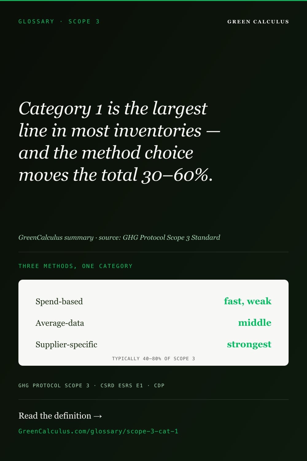
Scope 3 Category 1 covers cradle-to-gate emissions from all upstream goods and services a company buys — typically 40–80% of total Scope 3. Three GHG Protocol methods apply: spend-based, average-data and supplier-specific, in increasing order of strength.
What Category 1 Covers — and What It Does Not
Scope 3 Category 1 (“Purchased goods and services”) covers cradle-to-gate emissions from all upstream goods and services purchased or acquired by the reporting company in the reporting year. “Cradle-to-gate” means everything from raw-material extraction through manufacturing up to the point the goods arrive at the supplier’s gate — but not the transport to the reporting company (that is Cat 4 upstream transport) and not any subsequent use or disposal.
The category is intentionally broad. It includes physical goods (raw materials, components, packaging, office supplies, equipment for resale), services (consulting, legal, software-as-a-service, marketing agencies, cleaning, security), and intermediate inputs used in production. The defining test is whether the purchase is a non-capital good or service — capital goods (machinery, buildings, vehicles purchased for own use) sit in Cat 2 instead.
| Sector | Typical Cat 1 line items | Typical Cat 1 share of Scope 3 |
|---|---|---|
| Manufacturing | Raw materials, components, packaging, sub-assemblies, contract manufacturing | 50–80% |
| Food & beverage | Agricultural commodities, ingredients, packaging, co-packing services | 60–85% |
| Retail | Goods for resale (almost always the dominant line), private-label production | 70–90% |
| Financial services | IT services, professional services, office consumables (Cat 15 financed emissions usually dominates) | 5–20% |
| Technology / SaaS | Cloud services, contract development, hardware components, professional services | 30–60% |
| Healthcare / pharma | Active pharmaceutical ingredients, packaging, lab consumables, clinical research services | 40–65% |
| Construction | Cement, steel, glass, aggregates, subcontracted labour services | 60–85% |
Sector ranges are illustrative based on published CDP disclosures across 2023–2025 reporting cycles. Actual share varies by company size, integration level, and scope completeness.
Cat 1 vs Cat 2 (capital goods): the test is whether the purchase is capitalised on the balance sheet (Cat 2) or expensed as cost of goods or operating cost (Cat 1). Machinery, buildings, and vehicles purchased for own use go to Cat 2. Raw materials, components, and services consumed in the reporting year go to Cat 1.
Cat 1 vs Cat 4 (upstream transportation): Cat 1 covers the supplier’s gate-to-gate manufacturing. Cat 4 covers the inbound transport from the supplier to the reporting company when paid for separately. When transport is bundled into the purchase price (DDP Incoterms, included in unit cost), the transport portion is in Cat 1 by default and excluded from Cat 4 to avoid double counting.
Cat 1 vs Cat 3 (fuel- and energy-related activities): purchased fuels combusted on site go to Scope 1, with their upstream supply in Cat 3a. Cat 1 covers non-fuel purchased goods. Purchased electricity sits in Scope 2 with its upstream fuel in Cat 3b and grid T&D losses in Cat 3c.
Cat 1 vs Cat 11 (use of sold products): Cat 1 is upstream of the reporting company. Cat 11 is downstream — emissions when customers use the company’s sold products. They do not overlap.
The Three Calculation Methods — the Central Decision
The GHG Protocol Scope 3 Standard permits three calculation methods for Category 1, sitting on a data-quality hierarchy. The choice is not a yes/no decision — most mature Cat 1 inventories use a blend, applying the strongest available method to the largest spend categories and falling back to weaker methods only for the long tail.
| Method | Activity data | Emission factor source | Data quality (PCAF 1-5) | Effort |
|---|---|---|---|---|
| Spend-based | $ spent per supplier or category | EEIO factor (kg CO₂e per $) | Score 5 (weakest) | Low — days |
| Average-data | Physical quantity (kg, m², units) | Industry-average factor (kg CO₂e per unit) | Score 3 | Medium — weeks |
| Hybrid | Physical quantity where available + spend for the rest | Mix of supplier PCF, industry-average, and EEIO | Score 2-3 | Medium-high — months |
| Supplier-specific | Physical quantity | Supplier’s product carbon footprint (PCF) under ISO 14067 | Score 1 (strongest) | High — supplier engagement programme |
PCAF data quality scores per the PCAF Financed Emissions Standard, which has become the de facto data-quality language across Scope 3 (originally written for financed emissions but the 1-5 framework is widely adopted for value-chain categories). Score 1 = verified supplier-specific data; Score 5 = proxy data with no supplier engagement.
Data-quality progression — visualised
The bar chart below shows the typical inventory composition by data-quality score as a Cat 1 programme matures from year 1 (almost entirely spend-based) through year 5 (supplier-engaged on the top of the spend curve).
Green = supplier-specific (PCAF Score 1-2). Blue = average-data (Score 3). Amber = spend-based (Score 5). Illustrative trajectory; specific timing depends on supplier base size and engagement resources.
Spend-based Cat 1 has a structural problem beyond data quality: it does not respond to decarbonisation. When a supplier switches from grid electricity to renewable PPAs, their EEIO sector factor does not change for years — so the reporting company’s spend-based inventory shows no improvement even though the actual upstream emissions have fallen. SBTi target-tracking under the Corporate Net-Zero Standard requires supplier-specific data to count supplier decarbonisation against the target. Companies that stay spend-based effectively cannot claim Scope 3 reduction credit no matter what their suppliers do.
Spend-Based Method — EEIO Factors, Currency, Deflation
Spend-based Cat 1 multiplies the reporting company’s procurement spend in a given sector by an Environmentally-Extended Input-Output (EEIO) factor expressed as kg CO₂e per unit of currency. EEIO factors are derived from national input-output economic tables paired with industry-level emission inventories — the result is an average kg CO₂e per dollar (or euro, or pound) of output for each sector of the economy.
Three EEIO databases dominate practice:
| Database | Geographic scope | Currency basis | Typical use |
|---|---|---|---|
| USEEIO (EPA, USA) | United States, 411 sectors | USD, 2017 producer prices | US-domiciled companies, US procurement |
| Exiobase (NTNU et al.) | Global, 49 regions × 200 sectors | EUR, multiple base years | European and multinational disclosure |
| CEDA (Watershed et al.) | Global, 145 sectors | Multiple, refreshed annually | Commercial Scope 3 platforms |
The arithmetic and where it breaks
The calculation is straightforward: Cat 1 emissions = procurement spend × EEIO factor. A $5 million spend in the “Iron and steel mills” sector (USEEIO 331110) at approximately 1.6 kg CO₂e per 2017-USD produces 8,000 tonnes CO₂e for the line. The arithmetic is mechanical; the difficulty is in three places that practitioners miss.
(1) Spend categorisation. The procurement system records line items at supplier and account-code granularity, not at EEIO-sector granularity. Mapping ledger codes to the 200–411 EEIO sectors is manual and judgement-driven. The same line item can plausibly map to two or three EEIO sectors with a 2–3× spread in factor value — the mapping decision is often the single largest source of variance in the inventory total.
(2) Currency conversion. EEIO factors are denominated in a specific currency (USEEIO in USD, Exiobase in EUR). A UK or Singapore company applying USEEIO must convert GBP or SGD spend to USD at the appropriate exchange rate. Using current-year rates against a 2017-base factor introduces FX drift; using 2017 rates against current spend is internally consistent but loses cross-year comparability.
(3) Deflation to factor base year. EEIO factors are anchored to a base year (USEEIO is 2017). A $1 million spend in 2026 is not equivalent to a $1 million spend in 2017 in real economic activity — general inflation since 2017 means $1 million in 2026 buys roughly $0.77 million of 2017-equivalent output. Spend must be deflated to the factor’s base year using an appropriate price index (the Producer Price Index for the sector, or GDP deflator as a fallback). Failure to deflate over-states the inventory by the cumulative inflation rate since the factor base year — typically 25–35% for a 2017-base factor applied to 2026 spend.
Of the three EEIO problems above, deflation is the one most consistently missed. A spend-based Cat 1 inventory that uses 2026 nominal spend against a 2017 USEEIO factor and does not deflate is over-stating the inventory by approximately 30%. Worse, the over-statement grows every year — by 2030 the same un-deflated approach will be over-stating by approximately 40%. The fix is to apply a sector-specific Producer Price Index (PPI) deflator to convert nominal current-year spend to factor-base-year-equivalent spend before multiplying. The deflator step adds an hour to the inventory build; not adding it adds a 30%+ structural bias that grows annually.
Activity-Based and Supplier-Specific Methods
Average-data (activity-based) method
The average-data method replaces dollars with physical quantity — kilograms, square metres, units, kilowatt-hours — and pairs it with an industry-average emission factor expressed in kg CO₂e per physical unit. For commodities like steel, cement, paper, plastics, and aluminium, industry-average factors are published by sector associations and embodied in DEFRA, ecoinvent, or the WBCSD Pathfinder sector libraries. The factor avoids the currency and deflation problems of spend-based and is generally a step closer to true activity, but it is still a sector average — not the specific supplier the reporting company actually uses.
Average-data is the natural method when (a) the goods are commodities with well-defined physical units and (b) the supplier has not yet provided a PCF. It is the dominant method for cement, steel, primary aluminium, paper packaging, and bulk chemicals in mature Cat 1 inventories. The data-quality score is typically PCAF 3.
Supplier-specific method — product carbon footprints under ISO 14067
The strongest method uses a verified product carbon footprint (PCF) from the supplier, calculated under ISO 14067 and built on ISO 14040/14044 LCA principles. The supplier publishes (or shares confidentially) a kg CO₂e per unit value specific to their production process, energy mix, and supply chain — and the reporting company uses that value directly against the physical quantity purchased.
Supplier-specific Cat 1 has three properties that make it the SBTi-target-tracking gold standard. (1) It captures supplier-level decarbonisation: when the supplier switches to renewable energy, their PCF falls and the reporting company’s Cat 1 line falls in lockstep. Spend-based and average-data methods don’t see this. (2) It supports sector-specific differentiation: a low-carbon steel supplier (electric arc furnace + renewable power) produces a PCF 60–80% below the industry average, and supplier-specific accounting rewards the reporting company for sourcing from them. (3) It is the data-quality basis SBTi requires for Scope 3 target tracking under the Corporate Net-Zero Standard.
A PCF that is genuinely usable for Cat 1 accounting needs five elements: (1) a defined functional unit (“per kg of finished product”, “per kWh of electricity delivered”, “per litre of solvent”), (2) a clearly stated cradle-to-gate system boundary, (3) the underlying emission factor sources and reference year, (4) the GWP basis (AR6 is the corporate default), and (5) third-party verification or assurance statement. A PCF that lacks (5) can still be used but should be flagged in the methodology disclosure as supplier-self-reported. The emerging WBCSD Pathfinder Framework is standardising the PCF exchange format across industries — expect supplier-specific data to become substantially easier to obtain over 2026–2028.
Worked Example — Three Methods on One Procurement Portfolio
A mid-size manufacturing company spends $50M annually across five major Cat 1 categories. The table below applies all three calculation methods to the same procurement portfolio to show how the inventory total moves. All values are illustrative and hardcoded — substitute the company’s own EEIO factors, industry-average factors, and supplier PCFs in real use.
| Category | Spend ($M) | Physical qty | Spend-based tCO₂e | Average-data tCO₂e | Supplier-specific tCO₂e |
|---|---|---|---|---|---|
| Steel components | 15 | 8,500 t | 24,000 | 15,300 | 10,200 |
| Plastic resin | 10 | 3,200 t | 12,500 | 8,000 | 7,400 |
| Electronic assemblies | 12 | ~120k units | 18,200 | 14,800 | 11,500 |
| Packaging (paper + film) | 5 | 1,400 t | 6,800 | 4,200 | 3,800 |
| Professional services | 8 | n/a | 2,400 | 2,400 (no avg factor) | 1,900 (PCF avail.) |
| TOTAL Scope 3 Cat 1 | 50 | 63,900 | 44,700 | 34,800 | |
| Change vs spend-based baseline | baseline | −30% | −46% | ||
All values hardcoded — illustrative figures, not real factors. The 30–60% spread between spend-based and supplier-specific is consistent with published case studies across CDP 2024 disclosures. The pattern: spend-based produces the highest total (low-carbon suppliers do not appear different from the industry average), supplier-specific produces the lowest total (the company has actively sourced from below-average-intensity suppliers and gets credit for it). Average-data sits in between — better than spend, less responsive than supplier-specific.
The three columns are not “estimates of the same true value with different error bars.” They are three different things being measured. Spend-based answers “what would an industry-average dollar of this kind of procurement emit?” — a national-economic-average question. Average-data answers “what would the average unit of this physical commodity emit?” — a sector-average question. Supplier-specific answers “what did the actual suppliers we used actually emit?” — a company-specific question. As the methodology shifts, the question being asked sharpens. The “right” answer for SBTi target tracking is the supplier-specific one because it is the only column that responds to procurement decarbonisation decisions.
Build a defensible Scope 3 Cat 1 inventory with full methodology disclosure and supplier-engagement tracking.
The Same Purchase, Priced on Live Factors
The portfolio above is illustrative and says so. This section does the same comparison on one purchase with real factors, read from the data layer as this page loads. The result is more interesting than a gap: it shows that the spend-based figure is set largely by what you paid, not by what you received.
Take structural steel, bought in the United States. Two of the three rungs have a published factor.
| Rung | Factor, live | What it is keyed to | Publisher |
|---|---|---|---|
| Spend-based | 1.005215 kg CO2e per 2024 USD purchaser price | NAICS-6 331110, Iron and Steel Mills. A dollar of purchase. | USEEIO Supply Chain Factors v1.4.0, CC BY 4.0 |
| Average-data | 0.56029 kg CO2e per kg | Hot-rolled structural sections, EN 15804+A2 modules A1–A3. A kilogram of steel. | ÖKOBAUDAT 2024 Release I, CC BY 4.0 |
| Supplier-specific | — | This supplier’s product footprint for this order. | None, by design — see below. |
Both factors are fetched from the open endpoint when you press the button, so this never goes stale. Change the price and watch which number moves.
The physical quantity on the delivery note.
The invoice total. The default is illustrative — put your own in.
There is a price at which the two methods agree exactly. Below it the spend-based figure is the lower of the two; above it, the higher. Nothing about the steel changes as you cross that line — only the invoice. Negotiating a discount reduces a spend-based footprint. Buying the identical steel from a cleaner mill at a premium increases it. That is not a flaw in the factor, which is answering a question about dollars honestly. It is the reason the method sits at the bottom of the hierarchy, and the reason it cannot be used to track a decarbonisation target.
Average-data does not have that property. It is keyed to mass, so the same 100 tonnes gives the same answer whoever you bought it from and whatever you paid — which makes it stable, and equally makes it blind to any supplier you have deliberately chosen for being better than average. Only the top rung sees that, which is why the ladder ends where it does.
The rung does not decide the category. Our spend factor is filed under Category 1 and the ÖKOBAUDAT material factor under Category 2, capital goods — because the construction database it comes from describes materials going into buildings. The same steel is Category 1 if it becomes part of a product you sell and Category 2 if it becomes part of your own building. Decide the category from what the purchase is for, then choose a rung; never let the factor you happened to find decide the category for you.
The dollar year is part of the factor. That spend factor is per 2024 dollar. Applying it to 2022 spend overstates the result by whatever inflation ran in between. When the publisher moved this set from a 2022 to a 2024 denominator, 1,106 factors changed their unit without changing much of their number — the trap covered in how often emission factors change.
Why the top rung has no factor
The supplier-specific row above is empty and will stay empty. No database can hold it, because the whole point of the rung is that the number belongs to one supplier and one product rather than to an industry or a material. A factor database can tell you what an average tonne of steel emits; only your supplier can tell you what theirs did. That is the work the top rung asks for, and it is why moving up the hierarchy stops being a data problem and becomes a procurement one — the subject of the supplier-specific method and of supplier screening.
What a good data source can do is tell you honestly which rung a number came from. Every factor in the responses behind this page carries that: whether it is supplier-specific, what its activity basis is, and how representative it claims to be. Those fields are shown in full in anatomy of a traceable carbon number.
Materiality and Prioritisation — the Pareto Problem
Scope 3 Cat 1 inventories almost always exhibit a sharp Pareto distribution: the top 20% of suppliers (by emissions, not by spend) account for 70–85% of the total Cat 1 line. The implication for inventory development is operational: supplier engagement effort concentrates on the top of the curve, while the long tail can remain spend-based or average-data without meaningfully degrading total inventory accuracy.
Illustrative distribution — the exact split varies by sector. Manufacturing and food companies typically show sharper Pareto curves than retail or technology. Source: aggregated patterns across CDP Supply Chain disclosures 2023–2025.
Operational implications
The Pareto distribution dictates the year-one inventory architecture. A defensible Cat 1 build looks like this:
- Spend-categorise the entire portfolio — map every supplier and procurement category to an EEIO sector. Produces a complete spend-based estimate of total Cat 1.
- Rank suppliers by estimated emission contribution — combine spend with EEIO factor to identify the top-emitting suppliers (not the top-spending suppliers; a software vendor with $5M spend and a 0.04 kg CO₂e/$ factor is far below a steel supplier with $2M spend and a 1.6 kg CO₂e/$ factor).
- Engage the top 10–20% on PCF data — request supplier-specific PCFs from the suppliers that account for ~80% of the estimated total.
- Apply industry-average factors to the next tier where physical quantity data is available but supplier PCF is not.
- Leave the long tail at spend-based — the bottom 50% of suppliers by emissions accounts for less than 5% of the total; supplier engagement here is not a cost-effective use of effort and is often actively discouraged by mature programmes.
Under the CSRD/ESRS E1 double-materiality framework, the prioritisation is anchored to financial and impact materiality — the same Pareto principle expressed in regulatory language. Under SBTi the Supplier Engagement Target explicitly recognises that supplier engagement on 67%+ of relevant Scope 3 emissions (typically Cat 1 + Cat 11) is the metric being tracked — not 100% coverage, which is operationally infeasible.
Four Common Category 1 Reporting Mistakes
- Staying spend-based when supplier data is available. The most consequential error. A company that has received supplier PCFs from its top steel and chemicals suppliers but continues to apply USEEIO sector factors across the entire procurement portfolio is reporting an inventory that does not respond to its own decarbonisation choices. SBTi target tracking under the Corporate Net-Zero Standard requires supplier-specific data for hotspot suppliers to count their decarbonisation against the target. Spend-based-everywhere is an audit and target-credibility risk by 2026.
- Confusing Cat 1 (operating expense) with Cat 2 (capital goods). The boundary is whether the purchase is capitalised. Machinery, buildings, vehicles, IT hardware purchased for own use are Cat 2 regardless of how the procurement system tags them. Raw materials, components, consumables, and services consumed in the reporting year are Cat 1. The same supplier can be split across both categories — a packaging supplier might invoice both consumable packaging (Cat 1) and a packaging-line machine (Cat 2). Verify the accounting treatment, not the supplier identity.
- Not deflating spend to the EEIO factor’s base year. A 2017-base USEEIO factor applied to nominal 2026 spend without deflation over-states Cat 1 by approximately 30%. The error grows every year as inflation accumulates. The fix is a sector-specific Producer Price Index deflator, applied as a one-line multiplier before the EEIO factor. Most spend-based inventories built off-the-shelf from procurement-data extracts skip this step entirely. See §3 for the mechanics.
- Double-counting upstream transport across Cat 1 and Cat 4. When inbound transport is bundled into the supplier’s unit price (DDP Incoterms, “delivered duty paid”), the transport emissions are inside the spend-based EEIO factor or inside the supplier’s PCF and therefore in Cat 1. Adding a separate Cat 4 calculation on top double-counts the transport line. When inbound transport is invoiced separately (the reporting company pays the carrier directly), the transport is excluded from the unit price and belongs in Cat 4 alone. The Incoterm or invoicing arrangement determines which category the transport sits in — always check before adding a Cat 4 line on top of a Cat 1 baseline.
Dataset — the full factor set behind this term, versioned with source provenance and downloadable as CSV with a citable Zenodo DOI, is published as the UK spend-based GHG intensity by SIC section dataset.
Related Terms, Standards, and Tools
Frequently Asked Questions
Scope 3 Category 1 covers cradle-to-gate emissions from all upstream goods and services purchased by the reporting company in the reporting year. “Cradle-to-gate” means everything from raw-material extraction through manufacturing up to the supplier’s gate — but not transport to the reporting company (that is Cat 4) and not subsequent use or disposal. The category includes physical goods (raw materials, components, packaging, office supplies), services (consulting, legal, SaaS, marketing, cleaning), and intermediate inputs. The defining test is whether the purchase is a non-capital good or service — capital goods (machinery, buildings, vehicles for own use) sit in Cat 2 instead. Source: GHG Protocol Scope 3 Standard §5.1.
The boundary is capitalisation. Cat 1 covers purchased goods and services consumed in the reporting year — operating expense items. Cat 2 covers capital goods — machinery, buildings, vehicles, IT hardware purchased for the reporting company’s own use and capitalised on the balance sheet. The same supplier can split across both categories: a packaging supplier might invoice consumable packaging (Cat 1) and a packaging-line machine (Cat 2) in the same year. Verify the accounting treatment per line item, not the supplier identity. Under the GHG Protocol Scope 3 Standard, Cat 2 emissions are reported in the year of acquisition rather than amortised over the asset life.
The GHG Protocol Scope 3 Standard permits three methods on a data-quality hierarchy. Spend-based: multiply procurement spend by an EEIO factor (kg CO₂e per dollar) — fastest, weakest, PCAF data quality score 5. Average-data: multiply physical quantity (kg, units, m²) by an industry-average factor — medium effort, PCAF score 3. Supplier-specific: multiply physical quantity by a verified supplier product carbon footprint (PCF) under ISO 14067 — strongest, PCAF score 1. Mature inventories blend all three: supplier-specific for hotspot suppliers (typically top 10–20% by emissions), average-data for the middle tier, spend-based for the long tail. The three methods can produce inventory totals 30–60% apart on the same procurement portfolio — methodology disclosure is essential to tell readers which one they are looking at.
Spend-based multiplies procurement spend (dollars) by an EEIO sector factor (kg CO₂e per dollar) derived from national economic input-output tables. The factor reflects industry-average intensity for the sector, not the specific supplier’s performance. Supplier-specific multiplies physical quantity (kg, units) by a verified product carbon footprint (PCF) from the actual supplier, calculated under ISO 14067. The PCF reflects the specific supplier’s energy mix, production process, and supply chain. Three structural differences: (1) supplier-specific responds to supplier decarbonisation (renewable energy switch, process improvement) — spend-based does not; (2) supplier-specific allows low-carbon-supplier sourcing to show up in the inventory — spend-based treats all suppliers as average; (3) SBTi target tracking requires supplier-specific data for hotspot lines to count supplier decarbonisation against the target. Spend-based is the year-one starting point; supplier-specific is the year-five destination.
Because every company purchases substantially more upstream value than it produces directly. For a manufacturer, the embodied emissions of steel, aluminium, plastics, and components dwarf the energy emissions of the company’s own assembly operations — typically by 5–10×. For a retailer, the goods purchased for resale dominate the inventory: the company’s own stores and logistics account for <10% of total emissions and Cat 1 accounts for 70–90%. For food and beverage, agricultural commodities (especially livestock, dairy, and palm oil) have very high embodied intensities that compound through the supply chain. The two exceptions: financial services, where Cat 15 (Financed Emissions) dominates and Cat 1 is typically only 5–20%; and integrated energy and utilities, where Scope 1 combustion and Scope 3 Cat 11 (use of sold products) dominate. For every other sector, Cat 1 is the centre of gravity of the Scope 3 inventory — and the centre of gravity of the decarbonisation programme that follows.
Build Scope 3 Category 1 with method-appropriate data — supplier-specific where it matters, average-data for the middle, spend-based for the long tail. Methodology disclosure as audit-grade as the calculation itself.
Need someone who does this? 6 carbon accounting & inventory providers in our directory →