
Scope 3 Category 9 Downstream Transport & Distribution Calculator — GLEC Road, Sea, Air & Rail Freight Factors (tonne-km)
Compute Scope 3 Category 9 emissions for the distribution of your sold products — road, sea, air, rail, and inland waterway legs on GLEC Framework v3.2 well-to-wheel factors — in CO₂e on an IPCC AR6 GWP-100 basis, with the Category 4-versus-Category 9 boundary tested per leg.
The boundary call comes first. This calculator computes Scope 3 Category 9 — the transport and distribution of your sold products in vehicles and facilities you neither own nor pay for. Whether a given freight leg is Category 9 at all depends on who pays for it: transport you purchase, directly or indirectly, is Category 4 upstream; transport of sold products you do not pay for is Category 9. The tool asks who pays for each leg before it counts it, and shows any leg it routes to Category 4 in a separate note rather than silently dropping it.
You describe each leg; the engine picks the factor. Per leg you enter the mode (road, sea, air, rail, inland waterway), the vehicle or vessel profile, the distance, and the load — tonnes for most modes, TEU for sea containers. The engine looks up the well-to-wheel intensity live from MasterBrain by mode, profile, and region, multiplies by the activity, assigns a data-quality score, and rolls the legs into one Category 9 total. You never type a factor.
Two unit families, kept apart. Most modes are measured in tonne-kilometres — tonnes of freight times the distance moved. Sea container shipping is measured in TEU-kilometres — twenty-foot-equivalent units times distance — a different unit that the engine never sums against tonne-km. The two families produce the same kilograms of CO₂e, so they add cleanly at the output even though their activity units never mix.
Well-to-wheel, on an AR6 basis. Each GLEC factor is a well-to-wheel figure: the upstream fuel production emissions (well-to-tank) plus the combustion emissions (tank-to-wheel) in one number. The tool reports on the IPCC AR6 GWP-100 basis as a single CO₂e aggregate. A leg that draws on a DEFRA vehicle-kilometre factor or a storage facility shifts the inventory to a mixed-vintage basis, which the tool flags rather than hides.
GLEC Framework v3.2 (freight, tonne-km / TEU-km · AR6) + DEFRA 2026 (vehicle-km + WTT · AR5) + CIBSE TM46 (UK facility energy) + IPCC AR6 (refrigerants). Reads MasterBrain V3 live.
Add a downstream leg or facility above and click Calculate
Results appear with a freight / storage / retail component split, allocation sensitivity, per-line breakdown, data-quality scoring, reduction levers, audit trail, and export.
Results are indicative and for organisational greenhouse-gas accounting under the GHG Protocol Scope 3 Standard (Category 9). GLEC Framework v3.2 freight intensities are well-to-wheel (AR6 GWP-100, aggregate CO₂e with no per-gas decomposition); DEFRA 2026 delivery-vehicle factors are tank-to-wheel with a separately-published well-to-tank companion (AR5). Storage and retail use CIBSE TM46 typical UK benchmarks — replace with metered data where available, and note that non-UK facilities require metered energy. Storage and retail energy is apportioned to your goods by the allocation basis you select; record the basis and rationale. Verify the boundary (Category 4 vs 9), allocation, and distance basis against your value-chain data before external reporting; for assured disclosure obtain third-party verification under ISO 14064-3.
A manufacturer sells a pallet of goods ex-works. A container line carries it across an ocean, a haulier trucks it inland, and a retailer’s own van runs the last mile — none of it in a vehicle the manufacturer owns, none of it on a freight bill the manufacturer pays.
Every one of those legs is still the manufacturer’s emissions to report — but only the ones it doesn’t pay for, and only on the downstream side of the sale.
Category 9 is the emissions of distributing your sold products in vehicles you don’t own and don’t pay for. Transport you pay for is Category 4 instead. Count tonne-kilometres by mode, on a well-to-wheel, AR6 basis. Who pays sets the boundary.

What the Downstream T&D calculator covers
This calculator computes Scope 3 Category 9: the transport and distribution of your sold products — by road, sea, air, rail, and inland waterway — in vehicles and facilities you neither own nor control, and which you do not pay for. You describe each freight leg; the engine classifies it, picks the well-to-wheel factor for its mode, and sums the legs into a Category 9 total.
Why distributing a sold product is the seller’s downstream emission
Once a product is sold, it still has to reach the buyer, and the journey burns fuel in the seller’s name even though the seller has handed the goods on. Category 9 is the GHG Protocol’s answer to that journey: the distribution of sold products after the point of sale, in transport the reporting company doesn’t operate. The defining condition is payment — Category 9 captures the legs the seller does not pay for, because the legs it does pay for are accounted upstream in Category 4. The category exists to bring the downstream, unpaid distribution of sold goods back into the seller’s inventory.
Category 9 is not “all the freight after our gate.” It is specifically the distribution of sold products that the reporting company does not pay for. The transport you pay for — even outbound, even after the sale — is Category 4. The payment question decides the category before any factor is applied.
The modes
The calculator handles five freight modes, each with its own profile set. Road covers vans, rigid trucks, and articulated lorries by weight band, region, and fuel. Sea splits into the tonne-kilometre vessel classes — bulk carriers, tankers, general cargo, RoRo — and the container trade lanes, measured in TEU-kilometres. Air covers belly-hold and dedicated freighter, by haul length. Rail covers diesel and electric traction by region and commodity profile. Inland waterway covers barge and motor-vessel configurations. Each leg is entered separately, so the total is the sum of journeys you can name.
What’s in, what’s a separate category
| Covered in this calculator | Out of scope — separate category |
|---|---|
| Distribution of sold products in third-party transport the reporting company does not pay for — the downstream, unpaid leg | Transport the reporting company pays for, inbound or outbound — that is Category 4, upstream transport and distribution, regardless of when in the chain it occurs |
| Road, sea, air, rail, and inland-waterway legs of the sold-product journey to the end customer | Transport in vehicles the company owns or operates — that is the company’s own Scope 1 mobile combustion, not Category 9 |
| Retail and storage of sold products in third-party facilities, where the calculator supports a facility-energy line | The energy used at the product’s point of use by the consumer — that is Category 11, use of sold products, a separate accounting |
| The well-to-wheel emissions of each freight leg — upstream fuel plus combustion, in one figure | Assets the company leases out, or operations it franchises — Categories 13 and 14, accounted on the operator’s activity, not the freight of sold goods |
The boundary decision — Category 9 or Category 4
This is the page’s signature point, and the thing that makes Category 9 harder than multiplying tonne-kilometres by a factor. The same physical freight leg can be Category 9 or Category 4 — and which one it is depends not on the leg but on who pays for it. The tool runs the test per leg and shows its working.
The payment test
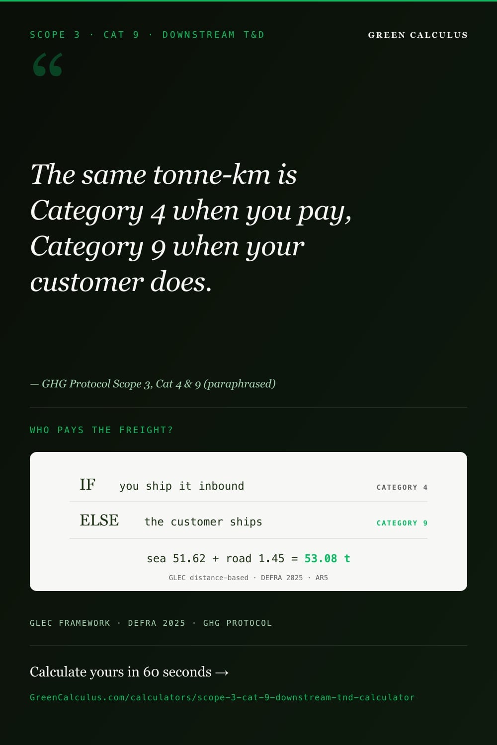
The GHG Protocol draws the upstream–downstream line for transport not by direction of travel but by who bears the cost. Transport the reporting company purchases — directly, or indirectly through the price it pays a supplier or carrier — is Category 4, upstream transport and distribution, whoever’s goods it moves and whichever way they travel. Transport of the company’s sold products that the company does not pay for is Category 9, downstream transport and distribution. A single outbound shipment can therefore land in either category: pay for it and it is Category 4; let the buyer pay and it is Category 9.
Sold-product distribution the seller doesn’t pay for
The cleanest Category 9 case is the product sold ex-works or free-on-board, where the buyer arranges and pays for onward carriage. The seller has no freight invoice, but under the GHG Protocol the downstream distribution of its sold product is still its value-chain emission — reported in Category 9, estimated where the seller lacks the buyer’s shipment data. For a manufacturer selling through distributors and retailers, Category 9 is frequently the larger and harder-to-source half of its outbound logistics footprint, precisely because the data sits with parties it doesn’t invoice.
The same container moving the same goods the same distance is Category 4 for a seller who pays the freight and Category 9 for a seller who doesn’t. Neither is wrong — they are answering the payment question differently. The calculator asks who pays for each leg and classifies it against the answer, so the category each leg lands in is a consequence of the commercial terms, not a guess.
The Incoterms wrinkle
Cutting across the payment question are the Incoterms that set who pays for which leg of a sale. Terms like EXW (ex-works) and FOB (free-on-board) leave the buyer paying for the main carriage, so the outbound legs are the seller’s downstream Category 9. Terms like DAP (delivered-at-place) and DDP (delivered-duty-paid) leave the seller paying through to destination, so the same legs become the seller’s upstream Category 4. Reading the Incoterm is the practical way to answer the payment test: it is the contractual record of who pays for transport, and therefore of where each leg belongs.
Do not classify a freight leg by direction alone. Outbound does not mean Category 9, and inbound does not mean Category 4 — the payment, set by the Incoterm, decides it. A DDP outbound shipment the seller pays for is Category 4; an EXW outbound shipment the buyer pays for is Category 9. Routing every outbound leg to Category 9 by reflex misplaces the ones the seller actually paid for.
A freight leg is Category 9 when it distributes a sold product, in transport the reporting company neither operates nor pays for. Change who pays — change the Incoterm — and the same leg becomes Category 4. The truck never moved.
This is also the most common place an inventory double-counts across companies. The leg you report as Category 9 — your sold product, carried on terms where the buyer pays — is the same leg your buyer may report as its Category 4 upstream transport. That is expected: one journey, two value chains, counted once on each side. The error is intra-company: counting a leg you pay for in both your Category 4 and your Category 9, or counting an owned-fleet leg in Category 9 when it belongs in your Scope 1.
Do not count a freight leg in both Category 4 and Category 9. A leg you pay for is Category 4; a leg you don’t pay for, distributing a sold product, is Category 9 — one or the other, never both. The tool’s per-leg reclassification note exists to make that single placement visible, so a leg can’t quietly appear in two categories of the same inventory.
Distance-based, fuel-based, or spend-based — choosing your method
Once a leg is confirmed as Category 9, the question is how to quantify it. The GHG Protocol gives three methods for transport, and the right one depends on the data the seller can actually get for freight it doesn’t control.
Distance-based (tonne-km)
Mass of goods times distance moved, multiplied by a mode-and-vehicle well-to-wheel intensity. The GLEC tonne-kilometre method, and the calculator’s primary path. The most practical route for sold-product distribution, because tonnage and route are usually knowable even when the seller doesn’t pay the freight.
Fuel-based
Litres or kilograms of fuel consumed on the leg, multiplied by a fuel emission factor. The most accurate method where the carrier can report actual fuel use for the shipment — rare in downstream distribution the seller doesn’t control, but the strongest data when available.
Spend-based
Freight spend, or an estimate of it, multiplied by an economic intensity for the transport service. The fallback when neither tonnage-and-distance nor fuel is available — and the weakest by data quality, since cost is a loose proxy for emissions. Used to close gaps, not as the default.
Mixed shipments
Real distribution chains mix methods: a tonne-kilometre estimate for the ocean leg, a carrier’s fuel figure for a contracted haulier, a spend proxy for a region with no shipment data. Each leg carries its own method and data-quality score, and the total reports the mix rather than forcing one method across the chain.
Why tonne-kilometres is the working default
For freight the seller doesn’t pay for, fuel data is usually out of reach — the carrier has it, the seller doesn’t. Spend data is often missing too, because there is no invoice to the seller. What the seller can usually reconstruct is the mass shipped and the route, and that is exactly what the tonne-kilometre method needs: tonnes times distance times a published mode intensity. The calculator leads with this method because it is the one most Category 9 inventories can actually populate, and the GLEC Framework intensities behind it are built for precisely this mode-level estimation.
Treat the three methods as an accuracy ladder: fuel-based first where a carrier reports real consumption, tonne-kilometre second as the practical default, spend-based last to close gaps. A carrier’s measured fuel beats a modelled tonne-kilometre estimate, which beats a cost proxy. Record which legs rest on which method — the calculator scores them accordingly, and the disclosure should name the mix.
How the calculation works — shipments to CO₂e
Every leg runs the same pipeline: test who pays, confirm the mode, look up the well-to-wheel factor, compute the tonnes of CO₂e, score the data quality, and roll up. What changes between legs is the mode, the profile, and the activity unit.
What you enter, and what the engine derives
One question sits over every leg: who pays for it. Per leg you then enter the mode, the vehicle or vessel profile, the distance, the load — tonnes, or TEU for sea containers — and the method. Everything downstream is derived: the engine looks up the well-to-wheel intensity from MasterBrain by mode, profile, and region — you never type a factor — computes the per-leg tonnes of CO₂e, assigns the Category 9-versus-Category 4 classification, scores the data quality, and sums the legs. Any leg the payment test routes to Category 4 appears in its own note with the reason, so the reclassification is visible rather than silent.
The two unit families
Category 9 mixes units, and the engine keeps them straight. Most modes are tonne-kilometres — tonnes of freight times distance, times a per-tonne-kilometre factor. Sea container shipping is TEU-kilometres — twenty-foot-equivalent units times distance, times a per-TEU-kilometre factor. The two activity figures are never added together — a tonne-kilometre and a TEU-kilometre are not the same quantity — but each factor resolves to the same kilograms of CO₂e, so the legs sum cleanly at the output.
Tonne-kilometres and TEU-kilometres are different units and are never summed. A 20-tonne-km road leg and a 20-TEU-km container leg describe different amounts of freight work. The engine multiplies each by its own factor, then adds only the resulting kilograms of CO₂e. Any table or chart that places a TEU-km figure beside a tonne-km figure as if they were comparable is an error.
Answer the payment question honestly and per leg, then let the classifier work. The temptation is to assume every outbound leg of a sold product is Category 9 and skip the test — but that is what produces the Category 4/Category 9 double-count an auditor will find. The reclassification note isn’t friction; it’s the audit trail that shows each leg sits in one category only.
Worked example — a sea leg and a road leg into one total
This example runs two legs of one outbound shipment for a seller whose buyer pays the freight, so both legs are Category 9. They use different unit families — one TEU-kilometres, one tonne-kilometres — and sum into a single total. The mode intensities are GLEC Framework v3.2 values; the tonnages and distances are illustrative inputs.
Leg A — deep-sea container, per TEU-kilometre
A 40-TEU consignment carried 18,000 km on a deep-sea container service, on the distance-based method, at the GLEC industry-average dry-container intensity.
| Step | Calculation | Result |
|---|---|---|
| Activity (TEU-km) | 40 TEU × 18,000 km | 720,000 TEU-km |
| Apply container WTW factor | 720,000 TEU-km × 0.0717 kg CO₂e/TEU-km | 51,624 kg |
| Sea leg (well-to-wheel) | WTT 9.144 t + TTW 42.480 t | 51.624 tCO₂e |
Leg B — road artic, per tonne-kilometre
A 24-tonne load carried 600 km on an inland articulated-lorry leg, on the distance-based method, at the GLEC EU/SA 34–40 t articulated diesel intensity.
| Step | Calculation | Result |
|---|---|---|
| Activity (tonne-km) | 24 t × 600 km | 14,400 tonne-km |
| Apply artic diesel WTW factor | 14,400 tonne-km × 0.101 kg CO₂e/tonne-km | 1,454.4 kg |
| Road leg (well-to-wheel) | WTT 0.3312 t + TTW 1.1232 t | 1.4544 tCO₂e |
GLEC Framework v3.2 factors, IPCC AR6 GWP-100. Deep-sea dry container 0.0717 kg CO₂e per TEU-km; EU/SA 34–40 t articulated diesel 0.101 kg CO₂e per tonne-km. Both legs are downstream distribution of a sold product the seller does not pay for, so both classify to Category 9. GLEC v3.2 via MasterBrain v2026.203.
The two legs share no activity unit — one is TEU-kilometres, the other tonne-kilometres — and those quantities are never added. What adds is the kilograms of CO₂e each produces: 51.624 plus 1.4544 gives a Category 9 total of 53.0784 tCO₂e, which the tool displays as 53.1 t on its magnitude-aware rounding. Note the well-to-tank split: the upstream fuel share of both legs, 9.4752 t, is reported as a separate well-to-tank companion line — here 9.48 t — alongside the Category 9 figure under the GHG Protocol Scope 3 Standard, not folded into it.
The activity units never sum; only the CO₂e outputs do. Adding 720,000 TEU-km to 14,400 tonne-km produces a meaningless number — the two describe different freight work. The engine multiplies each activity by its own factor and adds the resulting tonnes of CO₂e. The well-to-wheel factor already contains both the well-to-tank and tank-to-wheel shares; the well-to-tank companion is reported separately, not added on top.
The freight factors by mode
The factors behind the distance-based method come from the GLEC Framework v3.2 — the logistics-emissions methodology that is conformant with the ISO 14083 transport-chain standard. Each headline value is a well-to-wheel intensity on the IPCC AR6 GWP-100 basis. Most modes are quoted per tonne-kilometre; sea container is quoted per TEU-kilometre and never mixed with the rest.
Road — by vehicle class and region
Road factors run per tonne-kilometre, by truck class, weight band, region, and fuel. Intensity falls as vehicles get larger and loads consolidate: an urban delivery run carries far more carbon per tonne-kilometre than a full articulated trunk leg. The example articulated-lorry intensity below, 0.101 kg CO₂e per tonne-kilometre, is the EU/SA 34–40 t diesel default.
Sea — tonne-km classes and TEU-km container
Sea is the deepest mode and carries the unit firewall. The non-container vessel classes — bulk carriers, tankers, general cargo, RoRo, refrigerated bulk — are quoted per tonne-kilometre, and intensity falls steeply with vessel size as economies of scale take hold. Container shipping is quoted per TEU-kilometre across trade lanes, dry and refrigerated. The example below, 0.0717 kg CO₂e per TEU-kilometre, is the GLEC industry-average dry-container figure.
The container per-TEU-kilometre figure and the bulk-vessel per-tonne-kilometre figures are different units. A container at 0.0717 per TEU-km cannot be compared like-for-like with a bulk carrier at, say, 0.005 per tonne-km — a TEU is a box of varying mass, a tonne is a tonne. The calculator keeps the two on separate inputs and never ranks them on one axis.
Air — belly-hold and freighter
Air factors run per tonne-kilometre by deck type and haul length, and they are an order of magnitude above surface modes. Belly-hold capacity in passenger aircraft and dedicated freighters differ, and the ranking is not uniform: belly-hold is lighter per tonne-kilometre than a freighter on short hauls but heavier on long hauls, where dense long-haul freighters win. The GLEC air figures are quoted without a radiative-forcing uplift; the contrail and high-altitude effects that the passenger air-travel datasets add as an option are not applied to freight here.
Rail — diesel and electric traction
Rail is among the lowest-carbon surface modes per tonne-kilometre. Diesel traction carries a fixed intensity by region and commodity profile; electric traction tracks the regional grid factor, so a rail leg on a clean grid can fall well below its diesel equivalent. Rail and inland waterway are the two modes a distribution chain shifts freight onto to cut its Category 9 intensity.
The intensity ranking across modes is the comparison worth seeing on a single axis — all per tonne-kilometre, so it is a clean like-for-like. Sea container is deliberately absent: its TEU-kilometre unit does not belong on this axis.
GLEC Framework v3.2 per-tonne-kilometre factors, IPCC AR6 GWP-100. Bars scaled to the long-haul belly-hold air figure. Long-haul air freight is roughly thirty times the per-tonne-kilometre carbon of rail — mode choice, not just distance, drives the downstream freight stream. Sea container (per TEU-km) is a different unit and is not on this axis. GLEC v3.2 via MasterBrain v2026.203.
The mode gap dwarfs the within-mode gap. Moving a tonne of sold product by air rather than rail multiplies its distribution carbon by an order of magnitude — far more than any choice of truck class or vessel size within a mode. For Category 9, the highest-leverage question is which mode carries the freight, before how efficiently each mode is run.
Well-to-wheel — what the factor includes
Each GLEC factor is a well-to-wheel figure, and knowing what that bundles in keeps a Category 9 inventory from either under- or double-counting the upstream fuel share.
Well-to-tank plus tank-to-wheel
A well-to-wheel intensity has two parts. The well-to-tank share is the emissions of producing and delivering the fuel before it is burned — extraction, refining, distribution. The tank-to-wheel share is the combustion itself, the emissions from burning the fuel to move the freight. GLEC publishes the headline factor as the sum of the two, so a single Category 9 figure already contains the upstream fuel emissions. In the worked example, the sea leg’s 0.0717 splits into 0.0127 well-to-tank and 0.0590 tank-to-wheel; the road leg’s 0.101 splits into 0.023 and 0.078.
| Leg | Well-to-tank | Tank-to-wheel | Well-to-wheel (headline) |
|---|---|---|---|
| Sea container (per TEU-km) | 0.0127 | 0.0590 | 0.0717 |
| Road artic (per tonne-km) | 0.023 | 0.078 | 0.101 |
GLEC Framework v3.2, kg CO₂e per activity unit (TEU-km for sea container, tonne-km for road), IPCC AR6 GWP-100. Well-to-tank + tank-to-wheel = well-to-wheel exactly. GLEC v3.2 via MasterBrain v2026.203.
The well-to-wheel factor already includes the well-to-tank share — do not add a separate upstream-fuel line on top of a well-to-wheel Category 9 figure. The calculator can surface the well-to-tank companion for transparency and for reporters who account it under Category 3, but it is a decomposition of the same number, reported alongside, never an addition to the Category 9 total.
Data quality and the activity-data hierarchy
The GLEC factors are published and fixed, so a Category 9 inventory’s accuracy lives almost entirely in the activity data and the method: whether you have the carrier’s fuel, a measured tonnage and distance, or only a spend proxy. The calculator scores each leg 1 to 5, and the reporting expectation is to use the most specific data available and to be explicit where you didn’t.
| Tier | Leg data | Typical source |
|---|---|---|
| Primary / fuel-based | Actual fuel consumed on the leg, from the carrier, times a fuel factor | Carrier fuel reports, GLEC-accredited carrier programmes, telematics shared by the operator |
| Distance-based (tonne-km) | Measured mass and route, times a GLEC mode-and-vehicle intensity | Shipment manifests, bills of lading, route distances, vehicle/vessel profile from the carrier |
| Spend-based / estimated | Freight spend or a modelled tonnage estimate, times an economic or default intensity, for legs with no shipment data | Sales records by region, default mode splits, freight-cost estimates where the seller doesn’t pay the invoice |
The highest-value improvement for most Category 9 inventories is getting shipment-level mass and distance into the sales-and-distribution data request, which converts a spend proxy into a defensible tonne-kilometre estimate. The second is engaging the largest carriers for actual fuel data on the highest-volume lanes, where a fuel-based figure replaces a modelled one on the biggest lines. The honest disclosure names which legs rest on carrier fuel data, which on modelled tonne-kilometres, and which on spend proxies.
Audit checklist — what gets flagged in Cat 9 assurance
Category 9 is a boundary-heavy category, and the recurring assurance findings cluster around category placement and unit discipline rather than arithmetic. Each below traces to a classification error, a unit error, or a coverage assumption.
01 — Paid freight booked to Category 9
Routing a leg the reporter pays for to Category 9. Transport the company pays for is Category 4, whichever direction it travels. Only sold-product legs the company does not pay for are Category 9. Check the Incoterm.
02 — Leg counted in both Cat 4 and Cat 9
Booking the same leg upstream and downstream. A leg is Category 4 or Category 9, never both. The reclassification note shows which, and the payment test is what decides it.
03 — Activity units summed across families
Adding tonne-kilometres to TEU-kilometres before applying factors. The two are different quantities; only the kg CO₂e outputs add. A combined activity figure across the two units is a unit error.
04 — Owned-fleet leg in Category 9
Counting distribution in the company’s own vehicles as Category 9. Owned or operated transport is the company’s Scope 1 mobile combustion, not a Scope 3 value-chain emission.
05 — Well-to-tank added on top of well-to-wheel
Adding a separate upstream-fuel line to a well-to-wheel Category 9 figure. The well-to-wheel factor already contains the well-to-tank share; the companion is a decomposition, reported alongside, not an addition.
06 — Mode or method undocumented
Reporting Category 9 without recording the mode split or the method per leg. Distance-based, fuel-based, and spend-based give different accuracies; the basis must be stated for the inventory to be auditable.
Reporting context — Scope 3, IFRS S2, CSRD E1, SECR, ISO 14083
Category 9 emissions feed the same disclosure regimes as the rest of the Scope 3 inventory. The thread across the frameworks below is that all of them expect the category boundary, the method, and the factor source disclosed — which is why the payment test and the distance-versus-spend distinction matter beyond the headline number.
| Framework | Role for Category 9 emissions | Disclosure cadence |
|---|---|---|
| GHG Protocol Scope 3 Standard | The accounting standard. Defines Category 9 downstream transport and distribution and its distance-, fuel-, and spend-based methods, and the upstream–downstream payment boundary. | Same as the company’s reporting cycle |
| GLEC Framework | The freight methodology and factor source. Provides the mode-by-mode well-to-wheel intensities, the tonne-kilometre and TEU-kilometre allocation, and ISO 14083 conformance. | Periodic framework releases (v3.2 current) |
| UK DEFRA Conversion Factors | The supporting factor source for the vehicle-kilometre road path, the location-based grid factor behind storage and retail energy, and natural-gas combustion, on the AR5 GWP-100 basis. | Annual refresh (each DEFRA release) |
| IFRS S2 (ISSB) | The global disclosure baseline. Requires Scope 3 disclosure including downstream transport where material, with the method disclosed. | Annual, aligned with financial statements |
| CSRD ESRS E1 (EU) | The EU climate standard. ESRS E1 carries Scope 3 downstream-transport emissions in CO₂e as part of the gross Scope 3 total. | Annual sustainability statement |
| UK SECR | UK Streamlined Energy and Carbon Reporting. Downstream-transport emissions fall within voluntary Scope 3 scope; many reporters include them for a complete logistics footprint. | Annual, with the directors’ report |
For the reporting mechanics, the paired downstream transport methodology sets out the payment boundary, the distance- and fuel-based methods, and the GLEC factor sources in full. The underlying mode methodologies are documented in the GLEC road freight, sea freight, air freight, and rail freight methodologies, with last-mile delivery and cold-chain logistics covering the specialised legs.
Data sources, factors, and GWP basis
The factors — sources and structure
The distance-based method draws on the GLEC Framework v3.2 freight intensities — the logistics-emissions dataset spanning road, sea, air, rail, and inland waterway, conformant with the ISO 14083 transport-chain standard. Each headline value is a well-to-wheel intensity, quoted per tonne-kilometre for every mode except sea container, which is quoted per TEU-kilometre. The supporting paths — the vehicle-kilometre road option, the location-based grid factor behind any storage and retail facility line, and natural-gas combustion — draw on the DEFRA 2025 UK Government conversion factors. The full GLEC and DEFRA tables sit in the business travel and freight logistics factors reference and the DEFRA emission factors reference.
GWP basis
The page basis is IPCC AR6 GWP-100 as a single CO₂e aggregate, with no per-gas split and no toggle — the GLEC convention for its freight factors. This diverges from the DEFRA vehicle and energy factors used elsewhere on the site, which are on the AR5 basis. A pure-GLEC Category 9 calculation is therefore cleanly AR6. The moment a leg draws on a DEFRA vehicle-kilometre factor or a storage facility line, the inventory becomes mixed-vintage, and the calculator flags it as such rather than silently blending the two bases. For background on the assessment-report bases, see the IPCC AR6 GWP values reference and the global warming potential definition.
Coverage limits
Three coverage limits are worth naming plainly. First, the GLEC road intensities are regional — Europe and South America, China, North America, and India each have their own set, and a route in an unlisted region is best served by the nearest regional default with that noted. Second, sea container is the only mode quoted per TEU-kilometre, so a container leg cannot be priced on a tonne-kilometre basis without converting its load. Third, the air figures carry no radiative-forcing uplift; a reporter who wants to reflect high-altitude effects must add that adjustment outside the headline factor.
Versioning and update cadence
GLEC issues framework releases periodically and DEFRA refreshes its conversion factors annually, so both legs update on those cadences; the MasterBrain version against which a result was computed is stamped on the output, so a figure computed against one vintage and the same figure recomputed against a later one are distinguishable in restatement work. The downstream transport methodology documents the payment boundary and the factor sources in full.
What’s next — completing the transport picture
Downstream transport is one Category 9 line in a fuller value-chain picture. The adjacent calculators cover the paid, upstream side of the same freight, the specialised legs, and the organisational inventory that brings every scope together.
Live
Downstream Transport & Distribution
Distribution of sold products you don’t pay for, classified per leg and summed across modes. The calculator on this page.
Live
Cat 4 Road Freight & Sea Freight
The paid, upstream side of the same GLEC factor set — for the legs you pay for. Air, rail, last-mile, and cold-chain siblings round out the modes.
Live
ISO 14064-1 GHG Inventory
The organisational inventory roll-up across scopes, where the Category 9 total lands alongside Scope 1, 2, and the rest of Scope 3.
Roadmap
Downstream Leased Assets, Franchises & the Inventory Aggregator
Categories 13 and 14 and the Scope 1+2+3 aggregator. Methodologies live; calculators in build.
Live
GHG Inventory Aggregator
Roll Category 9 together with every other Scope 1, 2 and 3 source into one auditable corporate carbon footprint — the organisation-level inventory this category feeds into.
Live
Cat 10 Processing of Sold Products
Intermediate products your customers process further before final use, booked separately from their end use.
For the full methodological treatment — the payment boundary, the distance- and fuel-based methods, and the GLEC factor sources — see the downstream transport methodology. The air-freight, last-mile, and cold-chain legs of a distribution chain are covered by the air freight, last-mile delivery, and cold-chain logistics calculators, which share this page’s factor set on the paid, upstream side. For the owned-fleet contrast — distribution in vehicles the company runs itself — the Scope 1 and diesel references explain why an owned-fleet leg is a direct emission rather than a Category 9 one.
Frequently asked questions
It depends on who pays for the transport, not on its direction. Transport the reporting company pays for — directly or through a supplier’s price — is Category 4, upstream transport and distribution, whichever way it travels. Transport of the company’s sold products that the company does not pay for is Category 9, downstream transport and distribution. The Incoterm is the practical test: EXW or FOB leaves the buyer paying the outbound leg, making it the seller’s Category 9; DAP or DDP leaves the seller paying, making it Category 4.
A tonne-kilometre is one tonne of freight moved one kilometre — the standard activity unit for road, rail, air, inland waterway, and non-container sea freight. A TEU-kilometre is one twenty-foot-equivalent container moved one kilometre, the unit GLEC uses for sea container shipping. They are different quantities and are never summed: a TEU is a box of varying mass, a tonne is a tonne. The calculator multiplies each by its own factor and adds only the resulting kilograms of CO₂e.
For each leg of a sold product’s distribution that you don’t pay for, multiply the freight activity by a mode emission factor. The distance-based method takes tonnes times kilometres times a GLEC per-tonne-kilometre intensity (per-TEU-kilometre for sea containers). The fuel-based method takes a carrier’s actual fuel use times a fuel factor. The spend-based method takes freight cost times an economic intensity. Sum the kilograms of CO₂e across legs for the Category 9 total.
All three GHG Protocol transport methods. The distance-based method multiplies mass and distance by a GLEC well-to-wheel intensity by mode — the practical default. The fuel-based method multiplies a carrier’s actual fuel consumption by a fuel factor — the most accurate where available. The spend-based method multiplies freight spend by an economic intensity — the fallback for legs with no shipment data. They form an accuracy ladder: fuel-based strongest, spend-based weakest.
Road, sea, air, rail, and inland waterway. Road covers vans, rigid trucks, and articulated lorries by weight band, region, and fuel. Sea splits into tonne-kilometre vessel classes and TEU-kilometre container trade lanes. Air covers belly-hold and freighter by haul length. Rail covers diesel and electric traction by region and commodity. All run on GLEC Framework v3.2 well-to-wheel intensities.
Well-to-wheel is the full lifecycle of the fuel used on a leg: the well-to-tank share — producing and delivering the fuel — plus the tank-to-wheel share — burning it to move the freight. The GLEC headline factor is the sum of both, so a Category 9 figure already contains the upstream fuel emissions. The calculator can show the well-to-tank companion separately for transparency, but it is a decomposition of the same number, never an addition on top of the well-to-wheel total.
Because the category depends on who pays, and that differs by company and contract. The same container is the seller’s Category 9 when the buyer pays the freight, and the buyer’s Category 4 upstream transport on the same leg. One journey, two value chains, counted once on each side. The error is intra-company — counting a leg you pay for in both your own Category 4 and your own Category 9. The calculator asks who pays per leg and classifies against the answer.
AR6 GWP-100, as a single CO₂e aggregate with no per-gas split and no toggle — the GLEC convention for its freight factors. This diverges from the DEFRA vehicle and energy factors used elsewhere, which are on the AR5 basis. A pure-GLEC Category 9 calculation is cleanly AR6. If a leg draws on a DEFRA vehicle-kilometre factor or a storage facility line, the inventory becomes mixed-vintage and the calculator flags it rather than blending the bases silently.
Estimate it. Category 9 covers sold-product distribution the seller doesn’t pay for, so the seller often lacks the buyer’s shipment detail. Reconstruct the mass shipped and the likely route from sales records and default mode splits, apply the distance-based tonne-kilometre method, and score the leg’s data quality accordingly. Where even that isn’t possible, a spend-based estimate from freight cost closes the gap. The disclosure should name which legs are modelled rather than measured.
Per tonne-kilometre, long-haul air freight is roughly thirty times the intensity of rail and far above sea. Moving mass through the air takes far more energy than rolling it on rails or floating it on water, and the gap between modes dwarfs any efficiency difference within a mode. For Category 9, the mode that carries the freight is the highest-leverage decarbonisation question — shifting freight off air and onto rail, sea, or inland waterway cuts its distribution carbon by an order of magnitude.
Methodology notes and limitations
Scope and boundary. This calculator covers downstream transport and distribution under GHG Protocol Scope 3 Category 9 — the distribution of sold products in vehicles and facilities the reporting company neither owns nor pays for. Transport the company pays for, inbound or outbound, is Category 4; transport in owned or operated vehicles is the company’s Scope 1. The payment question, set in practice by the Incoterm, decides the category. The tool tests who pays per leg and surfaces any leg it routes to Category 4.
Three methods in this version. The distance-based method uses mass times distance times a GLEC mode-and-vehicle well-to-wheel intensity — the practical default. The fuel-based method uses a carrier’s actual fuel consumption times a fuel factor — the most accurate where the carrier reports it. The spend-based method uses freight spend times an economic intensity — the fallback for legs with no shipment data, and the weakest by data quality.
Two unit families. Most modes are quoted per tonne-kilometre; sea container is quoted per TEU-kilometre. The two activity figures are never summed — they describe different freight work — but each resolves to kilograms of CO₂e, so the legs add at the output. A combined activity figure across the two units is a unit error.
Well-to-wheel basis. Each GLEC factor is a well-to-wheel figure: well-to-tank fuel production plus tank-to-wheel combustion in one number. The well-to-tank companion can be reported separately for transparency or for Category 3 accounting, but it is a decomposition of the headline factor, never added on top of the well-to-wheel Category 9 total.
GWP basis. The page basis is IPCC AR6 GWP-100, a single CO₂e aggregate with no toggle — the GLEC convention. This diverges from the AR5 DEFRA factors used for the vehicle-kilometre road path and any storage or retail energy line; a leg using those flips the inventory to a mixed-vintage basis, which the calculator flags rather than blends.
Coverage limits. The GLEC road intensities are regional (EU/SA, China, North America, India); sea container is the only per-TEU-kilometre mode; and the air figures carry no radiative-forcing uplift. A route in an unlisted region uses the nearest regional default with that noted.
Activity data carries the accuracy, and no assurance opinion is given. The GLEC factors are fixed published values, so the result’s accuracy depends on the activity figures, the method, and the payment classification entered per leg. The calculator takes those as entered and does not independently verify them; the user is responsible for the activity-data basis, the category placement, and documenting the source of each leg’s inputs. Results are estimates and do not constitute an assurance opinion. They should be reviewed by a qualified practitioner before use in IFRS S2 disclosures, CSRD ESRS E1 datapoints, UK SECR returns, or other regulatory submissions.