
Scope 3 Cat 4 Road Freight Calculator (GLEC + DEFRA)
Convert tonnage and distance into well-to-wheel financed road-freight emissions under the GLEC Framework v3.2, with region-specific truck-class intensities and diesel, electric, and bio-LNG fuel pathways.
Activity-based formula (per leg):
Freight emissions (kg CO₂e) = Mass (tonnes) × Distance (km) × WTW intensity (kg CO₂e per tonne-km)
The activity-data spine is the tonne-kilometre — one tonne of cargo carried one kilometre. The calculator multiplies cargo mass by leg distance to derive tonne-km, then applies the GLEC Framework v3.2 well-to-wheel (WTW) intensity for the selected truck class, load factor, and fuel. WTW is the headline basis: it sums the upstream fuel-production component (well-to-tank, WTT) and the combustion component (tank-to-wheel, TTW). Battery-electric rows carry the entire WTW intensity in the WTT (upstream-grid) component with TTW set to zero, because there is no tailpipe combustion.
Region selection. GLEC v3.2 publishes four regional road factor sets, and the calculator does not blend them. Europe and South America share one set (freight_detailed.road.eu_sa.*), keyed by truck class × load factor × fuel, plus four weight-band .summary defaults (van, urban truck, medium goods vehicle, heavy goods vehicle). North America uses the flat US EPA SmartWay segment shape (freight_detailed.road.na.*) — 14 segments such as truckload dry van, less-than-truckload, refrigerated, flatbed, tanker, drayage, and package. China and India each carry their own regional set. Select the region that matches where the transport leg physically occurs, not where the shipper is domiciled.
Load factor (laden %). For the EU/SA set the result is highly sensitive to the load factor. An empty backhaul carries the vehicle’s fuel burn over zero payload, so the per-tonne-km intensity climbs sharply. The calculator exposes 0%, 50%, 100%, and an average laden option per class; enter the average laden state across the leg where the precise figure is unknown, and treat the empty-running portion explicitly where the operation runs dedicated backhauls.
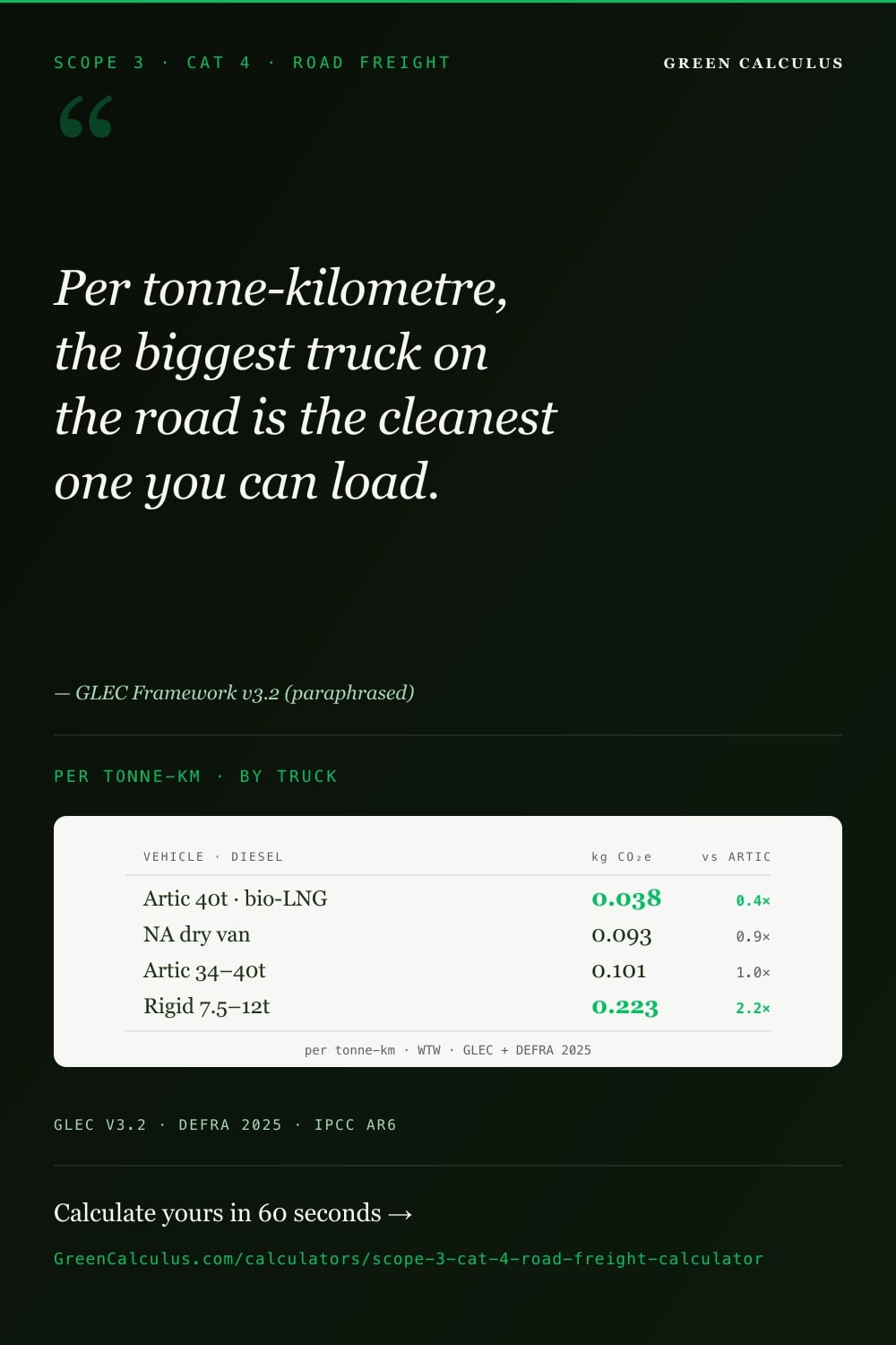
WTT/TTW split. The calculator renders the live WTW intensity for each class. The upstream/tailpipe decomposition (WTT and TTW) is published by GLEC alongside each row but is reported here as a fixed component pair in the worked example rather than a live field — it does not vary with the user’s inputs. For an artic 34–40t diesel tractor the WTW intensity of 0.101 kg CO₂e/tonne-km decomposes as 0.023 WTT + 0.078 TTW.
Fuel pathway. Diesel is the default. The EU/SA set also carries battery-electric and bio-LNG pathways for selected classes. Electric road freight is not zero-carbon on a WTW basis — its intensity is entirely the upstream grid emissions of the charging electricity, which for a rigid 12–20t in the EU/SA set is 0.22 kg CO₂e/tonne-km, higher than the equivalent diesel tractor on the same payload. Bio-LNG is the lowest-carbon pathway in the set at 0.038 kg CO₂e/tonne-km for an artic 34–40t spark-ignition engine. The fuel choice is a per-leg input, not a portfolio-wide assumption.
Category boundary. This calculator covers upstream transport and distribution (GHG Protocol Scope 3 Category 4) by road. The same GLEC road factors apply to downstream distribution under Category 9 — the arithmetic is identical, only the category label and the direction of the goods flow differ. Sea, air, rail, inland-waterway, last-mile, and cold-chain road freight each use their own factor sets and are out of scope for this tool.
GLEC Framework v3.2 (tonne-km, WTW · AR6) + DEFRA 2026 (vehicle-km, TTW + WTT companion · AR5). Reads MasterBrain V3 live.
Add a road leg above and click Calculate
Results appear with a well-to-tank / tank-to-wheel split, per-leg breakdown, data-quality scoring, low-carbon switch scenarios, audit trail, and export.
Results are indicative and for organisational greenhouse-gas accounting under the GHG Protocol Scope 3 Standard (Category 4). GLEC Framework v3.2 intensities are well-to-wheel (AR6 GWP-100); DEFRA 2026 delivery-vehicle factors are tank-to-wheel with a separately-published well-to-tank companion (AR5 GWP-100). GLEC freight CO₂e is published as an aggregate with no per-gas decomposition. Verify the boundary, allocation, and distance basis against your carrier data before external reporting; for assured disclosure obtain third-party verification under ISO 14064-3.
Road freight is the workhorse of almost every supply chain and the line item that turns a Scope 3 inventory from an estimate into an audit problem. Cargo moves across regions with different factor sets, trucks run half-empty on the backhaul, and a single supplier can ship the same pallet by diesel artic, battery-electric rigid, or bio-LNG tractor in the same quarter — each with a materially different carbon intensity per tonne-kilometre.
This calculator applies GLEC Framework v3.2 well-to-wheel intensities by region, truck class, load factor, and fuel — so the number you report is the number an assurer can trace.
Road-freight emissions equal cargo mass (tonnes) × distance (km) × the GLEC well-to-wheel intensity for the truck class, load factor, and fuel — summed across all legs. A laden artic 34–40t diesel tractor runs at 0.101 kg CO₂e per tonne-km.

What road freight covers in Scope 3 Category 4
GHG Protocol Scope 3 Category 4 — upstream transportation and distribution — covers the movement of purchased goods between a company’s tier-1 suppliers and its own operations, plus third-party logistics paid for by the reporting company. Road freight is the dominant mode within it for most organisations: the trucks that carry raw materials inbound and move stock between distribution centres.
Category 4 vs Category 9 — same factors, different direction
The distinction between Category 4 and Category 9 is the direction of the goods flow, not the calculation. Category 4 is upstream — transport the reporting company pays for, bringing goods in. Category 9 is downstream — transport of sold products after they leave the company’s control. The GLEC road intensities are identical across both; the calculator computes the emissions the same way, and the only editorial difference is which category line the result is booked to. A logistics provider reporting its own fleet emissions books them to Scope 1; a shipper paying that provider books the same tonne-km to Scope 3 Category 4.
Asset-class boundary — what’s in, what’s elsewhere
| Covered in this calculator | Out of scope — separate freight mode |
|---|---|
| Heavy goods vehicles — rigid and articulated, diesel, electric, or bio-LNG, across EU/SA, North America, China, and India | Sea freight — container, bulk, tanker, and RoRo vessels use per-tonne-km and per-TEU-km factor sets (separate calculator, in development) |
| Medium goods vehicles and urban trucks moving palletised freight between sites | Air freight — bellyhold and freighter jet-fuel intensities (separate calculator, in development) |
| Inter-site and trunking distribution by road | Rail freight — diesel and electric traction by commodity profile (separate calculator, in development) |
| Multi-region road legs of an intermodal journey (the road portions only) | Last-mile delivery — van and small-vehicle factors are per-kilometre, not per-tonne-km (separate calculator, in development) |
| Both diesel-default and alternative-fuel road tractors where the GLEC set carries the pathway | Cold-chain road freight — refrigerated transport adds a reefer-energy and refrigerant-leakage component (separate calculator, in development) |
Last-mile delivery and road freight are not the same calculation. Last-mile van factors are expressed per kilometre travelled, because parcel deliveries do not have a clean payload-tonnage denominator. Road freight is expressed per tonne-kilometre. Mixing the two — applying a per-km van factor to a tonne-km freight leg, or vice versa — produces a number that is wrong by orders of magnitude and is one of the most common errors an assurer catches.
How the calculation works — tonne-km × WTW intensity
Each leg of a road-freight movement reduces to one multiplication, run per leg and summed at the shipment or portfolio level:
Freight emissions (kg CO₂e) = Mass (tonnes) × Distance (km) × WTW intensity (kg CO₂e per tonne-km)
The activity-data spine — mass × distance = tonne-km
The tonne-kilometre is the unit that makes freight emissions comparable across modes and vehicles. Ten tonnes carried 100 km and one tonne carried 1,000 km are both 1,000 tonne-km and, on the same vehicle, carry the same emissions. The calculator takes cargo mass in tonnes and leg distance in kilometres as the two activity inputs; the product is the tonne-km the intensity factor multiplies. Where a journey has distinct legs — a 600 km trunk haul followed by a 40 km regional delivery on a smaller vehicle — each leg is entered separately with its own class and distance, because the intensity differs by vehicle.
Well-to-wheel, well-to-tank, tank-to-wheel
GLEC reports each road intensity as a well-to-wheel value — the full lifecycle of the fuel from extraction to combustion. It decomposes into two parts:
Well-to-tank (WTT)
The upstream emissions of producing and delivering the fuel before it reaches the vehicle — crude extraction, refining, and distribution for diesel; grid generation and transmission for electricity. See the well-to-tank definition for the full accounting boundary.
Tank-to-wheel (TTW)
The combustion emissions at the vehicle — the tailpipe CO₂e from burning the fuel in motion. For battery-electric vehicles this component is zero; the entire intensity sits in WTT as upstream grid emissions.
Why WTW is the headline
Scope 3 Category 4 requires the full upstream-and-combustion footprint of the transport service, so the WTW total is the figure that feeds the inventory. Reporting TTW alone — the tailpipe only — understates the freight footprint by the WTT share, which for diesel is roughly a fifth of the total.
Region selection — four sets, never blended
GLEC v3.2 carries four regional road sets, and the calculator keeps them separate. The selection axis differs by region: Europe and South America share a class × load × fuel matrix; North America uses a flat US EPA SmartWay segment shape. Select the region where the leg physically runs.
Choosing the right truck class and load factor
The two regional shapes ask for different inputs, and getting the class selection right is the difference between a defensible figure and a placeholder.
| Dimension | EU / South America | North America (SmartWay) |
|---|---|---|
| Key shape | road.eu_sa.<class>.<load>.<fuel> |
road.na.<segment>.diesel |
| Vehicle selection | Truck class (rigid 7.5–12t, rigid 12–20t, artic 34–40t, etc.) plus four weight-band .summary defaults |
Service segment (truckload dry van, less-than-truckload, refrigerated, flatbed, tanker, drayage, package) |
| Load factor | Explicit — 0%, 50%, 100%, or average laden | Embedded in the segment average — not a separate input |
| Fuel pathways | Diesel, battery-electric, bio-LNG (selected classes) | Diesel only |
| Typical intensity range | 0.038 (bio-LNG artic) to 0.223 (rigid 7.5–12t diesel) kg CO₂e/tonne-km | 0.093 (truckload dry van) to 1.272 (package) kg CO₂e/tonne-km |
The North American package segment running at 1.272 kg CO₂e/tonne-km is not an error — small-parcel networks carry low payload per vehicle-km relative to their distance, so the per-tonne-km intensity is an order of magnitude above trunk haulage. Where a North American leg is genuinely small-parcel, the package segment is correct; where it is full-truckload trunking, the truckload dry van segment at 0.093 kg CO₂e/tonne-km is the match.
Where the precise truck class is unknown — common when the leg is run by a third-party logistics provider who reports only mode and distance — use the EU/SA weight-band .summary defaults rather than guessing a specific class. The summary rows are GLEC’s published weight-band averages and are a defensible modelled default; a guessed specific class is not.
Diesel, electric, and bio-LNG — the fuel pathway comparison
For an articulated tractor in the 34–40t class moving the same payload over the same distance, the fuel pathway changes the per-tonne-km intensity by a factor of nearly six. The chart below compares the three EU/SA pathways for that class on a like-for-like payload basis.
Battery-electric road freight is not zero-carbon on a well-to-wheel basis, and on the current EU/SA grid mix it is not automatically lower than diesel. The 0.220 kg CO₂e/tonne-km electric figure is the upstream grid emissions of the charging electricity — its tank-to-wheel component is zero, but the whole intensity sits in well-to-tank. It is plotted here against a different vehicle class (rigid 12–20t electric vs artic 34–40t diesel) because the GLEC set does not carry an electric artic 34–40t row, so this is an illustrative cross-class contrast, not a same-vehicle swap. The reporting takeaway holds regardless: electrification reduces freight emissions only to the extent the charging grid is decarbonised, and a Scope 3 inventory must use the WTW figure, not a zero.
Bio-LNG is the lowest-carbon pathway in the set because the biogenic feedstock displaces fossil natural gas in the well-to-tank component. The GLEC intensity of 0.038 kg CO₂e/tonne-km reflects the lifecycle of the bio-LNG supply chain, not a zero-rating of the biogenic combustion — a distinction worth holding when reconciling against frameworks that treat biogenic CO₂ separately.
Why load factor decides the result
Within a single truck class and fuel, the load factor is the largest single driver of per-tonne-km intensity. A vehicle’s fuel burn is relatively insensitive to payload — an empty truck still burns most of the fuel a full one does — so spreading that burn over a smaller payload raises the per-tonne-km figure sharply. The chart below shows the effect for a representative rigid class across the GLEC laden states.
The chart is illustrative of the direction and magnitude of the effect rather than exact ratios, which vary by class. The practitioner consequence is concrete: a haulage operation that runs dedicated outbound loads and empty returns should account for the empty-running explicitly, because booking the whole journey at average laden understates the backhaul emissions. Where the operation balances loads in both directions, the average laden state is the appropriate default.
Load factor is the cheapest emissions lever in road freight and the one most often missing from supplier data. Asking a logistics provider for laden percentage alongside distance moves a leg from a modelled average to a measured value, and frequently reveals empty-running that backhaul optimisation can cut directly.
Worked example — a four-leg multi-region road shipment
This example reproduces against the live calculator. The shipment is a single consignment routed across two regions on three vehicle types and two fuels — the realistic shape of an intermodal supply leg where road handles the first and last segments. All factors are GLEC Framework v3.2 well-to-wheel intensities; the well-to-tank and tank-to-wheel components are shown where GLEC publishes them.
Inputs
| Leg | Region / class / fuel | Mass | Distance | WTW intensity |
|---|---|---|---|---|
| 1 — EU trunk haul | EU/SA · artic 34–40t · diesel | 22 t | 650 km | 0.101 kg CO₂e/t-km (WTT 0.023 + TTW 0.078) |
| 2 — EU regional | EU/SA · rigid 7.5–12t · diesel | 8 t | 120 km | 0.223 kg CO₂e/t-km (WTT 0.052 + TTW 0.172) |
| 3 — EU low-carbon shuttle | EU/SA · rigid 12–20t · electric | 12 t | 90 km | 0.220 kg CO₂e/t-km (grid upstream; TTW 0) |
| 4 — US final trunk | NA · truckload dry van · diesel | 18 t | 400 km | 0.093 kg CO₂e/t-km (WTT 0.016 + TTW 0.077) |
Leg-by-leg calculation
| Leg | Tonne-km | Intensity | Emissions (kg CO₂e) | Share |
|---|---|---|---|---|
| 1 — EU trunk haul | 22 × 650 = 14,300 | 0.101 | 1,444.3 | 53.3% |
| 2 — EU regional | 8 × 120 = 960 | 0.223 | 214.1 | 7.9% |
| 3 — EU electric shuttle | 12 × 90 = 1,080 | 0.220 | 237.6 | 8.8% |
| 4 — US final trunk | 18 × 400 = 7,200 | 0.093 | 669.6 | 24.7% |
| Total — Scope 3 Category 4 road freight | 2,565.6 | 94.7%* | ||
* Share column sums to 94.7% because the four leg shares are rounded to one decimal place; the underlying totals reconcile to 100%.
The 650 km EU diesel trunk haul dominates at 53.3% of the shipment footprint — long-distance, full-payload trunking carries the most tonne-km even at the lowest per-tonne-km intensity of the diesel legs. The electric shuttle, despite being the “low-carbon” leg, contributes 8.8% on only 1,080 tonne-km because its WTW intensity (grid upstream) is more than double the diesel artic’s. This is the reporting reality the WTW basis surfaces: the electric leg is not free, and over a short distance with modest payload it still books a non-trivial figure.
Shipment rollup
The blended shipment intensity of 0.109 kg CO₂e/tonne-km sits close to the diesel artic figure because the trunk haul dominates the tonne-km. Tracking this blended intensity over time is the cleanest decarbonisation signal for a road-freight programme — it isolates the carbon efficiency of the transport from the volume of goods moved, so a falling blended intensity reflects genuine modal or load-factor improvement rather than simply shipping less.
Data quality and the GLEC default hierarchy
GLEC frames freight data quality as a hierarchy from primary measured energy down to modelled defaults, and the calculator supports the full range. The reporting expectation is to climb the hierarchy where the emissions are material, not to apply the highest-precision method everywhere.
| Tier | Input shape | When it applies |
|---|---|---|
| Primary energy | Measured fuel or electricity consumed on the leg, converted via fuel factors | Own fleet, or a 3PL that shares metered fuel data — the most precise basis |
| Primary activity + modelled intensity | Actual mass and distance, with the GLEC class/load/fuel intensity | The default for most reporting — actual tonne-km, modelled factor. This calculator’s primary mode. |
| Modelled default | Actual mass and distance, with a weight-band .summary default where the class is unknown |
Third-party legs where only mode and route are known |
| Distance estimate | Estimated distance from origin–destination geocoding, modelled intensity | The fallback where even route distance is not supplied — flag as estimated |
The honest disclosure is the mix: a road-freight inventory that runs primary activity data on its top-20 lanes and modelled defaults on the long tail is a defensible, well-constructed inventory. Claiming primary-energy precision across every leg when most are modelled defaults is the disclosure failure, not the use of defaults itself.
Audit checklist — what gets flagged in freight assurance
Freight assurance under ISO 14083 and ISAE 3000 traces each leg from activity data to the rolled-up total. The findings below are the most common substantive issues raised on a road-freight inventory specifically.
01 — Per-km factor applied to a tonne-km leg
The reviewer-trap finding. A last-mile van factor (per kilometre) applied to a freight leg that should be per tonne-km, or the reverse. The two units differ by the payload tonnage and produce results wrong by an order of magnitude. Confirm the factor unit matches the activity unit on every leg.
02 — TTW reported instead of WTW
Reporting the tailpipe-only (tank-to-wheel) figure understates the freight footprint by the upstream fuel-production share — roughly a fifth for diesel. Scope 3 Category 4 requires the full well-to-wheel intensity. Confirm the headline factor is WTW, not TTW.
03 — Electric road freight booked as zero
Battery-electric legs have zero tank-to-wheel emissions but carry their full intensity in well-to-tank as upstream grid emissions. Booking an electric leg at zero on a WTW inventory is a finding. Use the GLEC electric WTW intensity, which reflects the charging grid.
04 — Regions blended into one factor set
Applying the EU/SA factor set to a North American leg, or averaging across regions, misstates the intensity — the SmartWay segment shape and the EU/SA class shape are not interchangeable. Each leg is factored against the region where it physically runs.
05 — Load factor defaulted to 100%
Assuming every leg runs fully laden ignores empty-running and understates the per-tonne-km intensity. Where actual load is unknown, the GLEC average-laden default is the defensible choice; 100% laden is only correct where the leg genuinely runs full.
06 — Distance basis undocumented
Whether distance is actual (telematics), planned route, or great-circle geocoded materially changes the tonne-km. The assurance team expects the distance basis documented per leg or per lane. Silently mixing actual and estimated distances without a flag is a finding.
Reporting context — Scope 3, GLEC/ISO 14083, IFRS S2, CSRD
Road-freight emissions feed several disclosure regimes through the same underlying GLEC calculation. The four frameworks below cover the disclosure surface a typical shipper or logistics provider navigates.
| Framework | Role for road-freight emissions | Disclosure cadence |
|---|---|---|
| GHG Protocol Scope 3 Standard | The accounting standard. Defines Category 4 (upstream transport & distribution) and Category 9 (downstream) as the lines for freight emissions and sets the activity-data and average-data method options. | Same as the institution’s reporting cycle |
| GLEC Framework v3.2 | The methodology standard for logistics emissions. Specifies the well-to-wheel intensities by mode, vehicle class, load factor, and fuel that this calculator applies. Now aligned with ISO 14083, the international transport-chain emissions standard. | Annual factor refresh |
| IFRS S2 (ISSB) | The global disclosure baseline. Requires Scope 3 disclosure including transport categories where material, with the calculation methodology disclosed. | Annual, aligned with financial statements |
| CSRD ESRS E1 (EU) | The EU sustainability-reporting mandate. ESRS E1 requires Scope 3 disclosure for in-scope companies, with transport and distribution among the categories assessed for materiality. | Annual sustainability statement |
GLEC and ISO 14083 — the convergence
The GLEC Framework and ISO 14083 have converged: GLEC v3.2 is structured to align with the ISO 14083 transport-chain emissions methodology, so a calculation built on GLEC intensities is also broadly ISO 14083-conformant. This matters for assurance — an ISO 14083 reference in a methodology statement signals an internationally standardised basis rather than a proprietary one, which assurers and disclosure regimes increasingly expect for transport emissions.
Data sources, factor versioning, and update transparency
Road intensities — source and structure
The road-freight intensities are drawn from GLEC Framework v3.2, retrieved for the MasterBrain factor set in May 2026. The set carries 125 road rows across four regions: Europe/South America (50 rows, class × load × fuel plus weight-band summaries), China (51 rows), North America (14 SmartWay segments), and India (10 rows). Each row’s headline value is the well-to-wheel intensity on an AR6 GWP-100 basis. The well-to-tank and tank-to-wheel components are published alongside each row and are reported in worked examples as fixed component pairs — they are not user-variable inputs. See the DEFRA emission factors reference for the UK road and fuel factors that complement the GLEC set for own-fleet legs.
GWP basis
The GLEC road set uses AR6 GWP-100 — the IPCC Sixth Assessment Report’s 100-year global warming potentials. This is the current GLEC convention and aligns with the GHG Protocol’s expected basis. Where a road-freight inventory is combined with DEFRA-sourced own-fleet legs, note that DEFRA factors are published on an AR5 GWP-100 basis; the calculator does not silently reconcile the two, and a mixed-basis inventory should disclose the mix rather than implying a uniform basis. See the global warming potential definition for the AR5-to-AR6 distinction.
Versioning and update cadence
GLEC publishes factor refreshes annually, and the MasterBrain factor set tracks each publication. The calculator stamps each result with the MasterBrain version against which it was computed, so a leg computed against one factor vintage and the same leg recomputed against a later vintage are distinguishable in restatement work. GLEC Framework version (v3.2) is independent of the underlying factor vintage — a methodology version applies across successive annual factor refreshes until the next framework revision ships.
What’s next — completing your Category 4 transport inventory
Road freight is the dominant mode in most upstream-transport inventories, but a complete Category 4 footprint spans every mode a supply chain uses. The other freight modes follow distinct factor sets — per-TEU-km for sea container, jet-fuel intensities for air, traction-and-commodity profiles for rail — and each requires its own calculator. The following modes are on the GreenCalculus build roadmap; none is published yet.
Live
Road Freight
GLEC v3.2 road set. Tonne-km × WTW intensity by region, class, load, and fuel. The calculator on this page.
Live
Sea freight
GLEC v3.2 sea set. Per-tonne-km for bulk, tanker, and RoRo; per-TEU-km for container — never mixed.
Live
Air freight
GLEC v3.2 air set. Bellyhold and freighter jet-fuel intensities by haul length.
Live
Rail freight
GLEC v3.2 rail set. Diesel and electric traction by commodity profile.
Live
Last-mile delivery
Van and small-vehicle factors — per kilometre, not per tonne-km. A different unit basis from road freight.
Live
Cold-chain logistics
Refrigerated freight adds a reefer-energy and refrigerant-leakage component on top of the transport intensity.
Live
GHG Inventory Aggregator
Roll Category 4 together with every other Scope 1, 2 and 3 source into one auditable corporate carbon footprint — the organisation-level inventory this category feeds into.
Live
Cat 9 Downstream Transport & Distribution
Transport and distribution of your sold products after they leave your gate — the downstream side of freight.
Separately from the upstream Category 4 modes above, downstream transport and distribution (the movement of sold products after they leave the company’s control) is accounted under Scope 3 Category 9, not Category 4. It uses the same GLEC road intensities but books to a different category line. A dedicated downstream transport calculator is on the roadmap and is not yet published.
Quick converter: g CO₂e/tonne-km to per tonne-mile.
Frequently asked questions
A tonne-kilometre is one tonne of cargo carried one kilometre. It is the activity unit for freight because it makes emissions comparable across vehicles and modes: ten tonnes carried 100 km and one tonne carried 1,000 km are both 1,000 tonne-km and, on the same vehicle, carry the same emissions. The calculator multiplies cargo mass in tonnes by leg distance in kilometres to get tonne-km, then applies the GLEC well-to-wheel intensity in kg CO₂e per tonne-km.
Well-to-wheel (WTW) is the full lifecycle of the fuel — production plus combustion. It splits into well-to-tank (WTT), the upstream emissions of producing and delivering the fuel before it reaches the vehicle, and tank-to-wheel (TTW), the combustion emissions at the vehicle. For a diesel artic 34–40t, the WTW intensity of 0.101 kg CO₂e/tonne-km is 0.023 WTT plus 0.078 TTW. Scope 3 Category 4 requires the WTW total; reporting TTW alone understates the footprint by the WTT share.
Battery-electric vehicles have zero tank-to-wheel (combustion) emissions, but their full intensity sits in well-to-tank as the upstream emissions of generating the charging electricity. On the current EU/SA grid mix, a rigid 12–20t electric runs at 0.220 kg CO₂e/tonne-km on a WTW basis — higher than an equivalent diesel artic. Electrification reduces freight emissions only to the extent the charging grid decarbonises, and a Scope 3 inventory must use the WTW figure, not a zero.
Load factor — the laden percentage — is the largest single driver of per-tonne-km intensity within a truck class. A vehicle burns most of its fuel whether full or empty, so spreading that burn over a smaller payload raises the per-tonne-km figure sharply. An empty backhaul has the highest intensity; a fully laden leg the lowest. Where actual load is unknown, the GLEC average-laden default is the defensible choice. Operations with dedicated empty returns should account for the empty-running explicitly.
Yes. The calculator carries the North American GLEC set built on the US EPA SmartWay segment shape — 14 segments including truckload dry van, less-than-truckload, refrigerated, flatbed, tanker, drayage, and package. North American legs use the segment selection rather than the EU/SA class-and-load-factor shape, with the load factor embedded in the segment average. Select the segment that matches the service type; for full-truckload trunking that is truckload dry van at 0.093 kg CO₂e/tonne-km.
The calculator computes the emissions identically for both — the GLEC road intensities are the same. The difference is the direction of the goods flow and the category line the result is booked to. Category 4 is upstream transport the reporting company pays for, bringing goods in. Category 9 is downstream transport of sold products after they leave the company’s control. Use this calculator for either; book the result to the correct category for your reporting boundary.
Use the EU/SA weight-band summary defaults — van, urban truck, medium goods vehicle, or heavy goods vehicle — rather than guessing a specific class. These are GLEC’s published weight-band averages and are a defensible modelled default for third-party legs where only mode and weight band are known. A guessed specific class is not defensible; a documented weight-band default is. Flag the leg as modelled-default in your data quality notes.
Bio-LNG’s biogenic feedstock displaces fossil natural gas in the well-to-tank component, so its lifecycle intensity is far below diesel — 0.038 kg CO₂e/tonne-km for an artic 34–40t spark-ignition engine versus 0.101 for the diesel equivalent. The GLEC figure reflects the full bio-LNG supply chain rather than a zero-rating of the biogenic combustion, a distinction worth holding when reconciling against frameworks that treat biogenic CO₂ as a separate line.
The GLEC road set uses AR6 GWP-100 — the IPCC Sixth Assessment Report’s 100-year global warming potentials, the current GLEC convention. Where road-freight legs are combined with DEFRA-sourced own-fleet legs, note that DEFRA factors are AR5 GWP-100; the calculator does not silently reconcile the two bases, and a mixed-basis inventory should disclose the mix rather than implying a uniform basis.
Yes. Distance drives tonne-km directly, so whether distance is actual (telematics), planned route, or great-circle geocoded materially changes the result. Actual route distance is the most accurate basis. Where only origin and destination are known, geocoded distance is a documented fallback — flag it as estimated. Assurance expects the distance basis documented per leg or lane; silently mixing actual and estimated distances is a finding.
Methodology notes and limitations
Methodology version. Calculator implements the GLEC Framework v3.2 road-freight intensities (retrieved May 2026), aligned with ISO 14083. Results are computed on an AR6 GWP-100 basis. Inventories computed against earlier factor vintages remain auditable against the corresponding MasterBrain version stamp.
Mode boundary. Road freight only — heavy and medium goods vehicles, rigid and articulated, across the four GLEC regional sets. Sea, air, rail, inland-waterway, last-mile, and cold-chain freight use separate factor sets and unit bases and are out of scope for this tool.
Unit basis. Intensities are per tonne-kilometre. This is distinct from the per-kilometre basis used for last-mile and small-vehicle delivery. The calculator does not convert between the two, and a per-km factor must never be applied to a tonne-km leg.
WTW headline; WTT/TTW fixed components. The calculator computes the well-to-wheel total. The well-to-tank and tank-to-wheel components are published by GLEC alongside each row and are reported in worked examples as fixed pairs; they do not vary with user inputs and are not separate live fields.
Electric and alternative fuels. Battery-electric intensities are the upstream grid emissions of the charging electricity (full intensity in WTT, TTW zero) and are not zero on a WTW basis. Bio-LNG intensities reflect the lifecycle of the bio-LNG supply chain. Both are per-leg fuel selections, not portfolio-wide assumptions.
Region not blended. The four regional road sets are kept separate. Each leg is factored against the region where it physically runs, and the EU/SA class shape and North American SmartWay segment shape are not interchangeable.
Activity data taken as entered. The calculator uses the mass, distance, and load factor the user enters; it does not independently verify them. The user is responsible for the activity-data basis — actual versus estimated distance, measured versus assumed load — and for documenting it per leg.
No assurance opinion. Results are estimates and do not constitute an assurance opinion. They should be reviewed by a qualified practitioner before use in IFRS S2 disclosures, CSRD ESRS E1 datapoints, or other regulatory submissions. The full methodological deep-dive — region-set selection trees, load-factor derivation, and the WTT/TTW decomposition — is published on the paired GLEC road-freight methodology page.